
文章目录[隐藏]
Ideal Sampling and Reconstruction
sampling theorem
If \(f(t)\) is a band-limited signal with a bandwidth of \(\omega_{m}\), the sampled spectrum \(F_{s}(\omega)\) of \(f(t)\) is the spectrum of \(f\). The spectrum \(F(\omega)\) is periodically extended on the frequency axis at intervals of the sampling frequency \(\omega_{s}\). Thus, when \(\omega_{s} \geq \omega_{m}\) frequency overlap does not occur; instead, it occurs when \(\omega_{s}<\omega_{m}\).
Model of Ideal Sampling
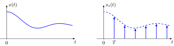
A continuous signal \(x(t)\) is sampled by taking its amplitude values at given time-instants. These time-instants can be chosen arbitrary in time, but most common are equidistant sampling schemes. The process of sampling is modeled by multiplying the continuous signal with a series of Dirac impulses. This constitutes an idealized model since Dirac impulses cannot be realized in practice.
For equidistant sampling of a continuous signal \(x(t)\) with sampling interval \(T\), the sampled signal \(x_\text{s}(t)\) reads
$$\begin{equation}
x_\text{s}(t) = \sum_{k = - \infty}{\infty} x(t) \cdot \delta(t - k T) = \sum_{k = - \infty}{\infty} x(k T) \cdot \delta(t - k T)
\end{equation}$$
where the multiplication property of the Dirac impulse was used for the last equality. The sampled signal is composed from a series of equidistant Dirac impulse which are weighted by the amplitude values of the continuous signal taken at their time-instants.
The series of Dirac impulse is represented conveniently by the Dirac comb. Rewriting the sampled signal yields
$$\begin{equation}
x_\text{s}(t) = x(t) \cdot \frac{1}{T} {\bot !! \bot !! \bot} \left( \frac{t}{T} \right)
\end{equation}$$
The process of sampling can be modeled by multipyling the continuous signal \(x(t)\) with a Dirac comb. The samples \(x(k T)\) for \(k \in \mathbb{Z}\) of the continuous signal constitute the discrete (-time) signal \(x[k] := x(k T)\). The question arises if and under which conditions the samples \(x[k]\) fully represent the continuous signal and allow for a reconstruction of the analog signal. In order to investigate this, the spectrum of the sampled signal is derived.
Reconstruction
Ideal Reconstruction deduction
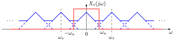
The question arises if and under which conditions the continuous signal can be recovered from the sampled signal. Above consideration revealed that the spectrum \(X_\text{s}(j \omega)\) of the sampled signal contains the unaltered spectrum of the continuous signal \(X(j \omega)\) if \(\omega_\text{u} < \frac{\omega_\text{s}}{2}\). Hence, the continuous signal can be reconstructed from the sampled signal by extracting the spectrum of the continuous signal from the spectrum of the sampled signal. This can be done by applying an ideal low-pass with cut-off frequency \(\omega_\text{c} = \frac{\omega_{s}}{2}\). This is illustrated in the following
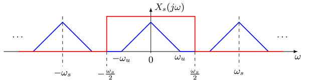
where the blue line represents the spectrum of the sampled signal and the red line the spectrum of the ideal low-pass. The transfer function \(H(j \omega)\) of the low-pass reads
$$\begin{equation}
H(j \omega) = T \cdot \text{rect} \left( \frac{\omega}{\omega_\text{s}} \right)
\end{equation}$$
Its impulse response \(h(t)\) is yielded by inverse Fourier transform of the transfer function
$$\begin{equation}
h(t) = \text{sinc} \left( \frac{\pi t}{T} \right)
\end{equation}$$
The reconstructed signal \(y(t)\) is given by convolving the sampled signal \(x_\text{s}(t)\) with the impulse response of the low-pass filter. This yields
$$\begin{align}
y(t) &= x_\text{s}(t) * h(t) \
&= \left( \sum_{k = - \infty}{\infty} x(k T) \cdot \delta(t - k T) \right) * \text{sinc} \left( \frac{\pi t}{T} \right) \
&= \sum_{k = - \infty}{\infty} x(k T) \cdot \text{sinc} \left( \frac{\pi}{T} (t - k T) \right)
\end{align}$$
where for the last equality the fact was exploited that \(x(k T)\) is independent of the time \(t\) for which the convolution is performed. The reconstructed signal is given by a weighted superposition of shifted sinc functions. Their weights are given by the samples \(x(k T)\) of the continuous signal. The reconstruction is illustrated in the following figure
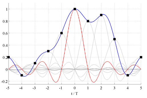
The black boxes show the samples \(x(k T)\) of the continuous signal, the blue line the reconstructed signal \(y(t)\), the gray lines the weighted sinc functions. The sinc function for \(k = 0\) is highlighted in red. The amplitudes \(x(k T)\) at the sampled positions are reconstructed perfectly since
$$\begin{equation}
\text{sinc} ( \frac{\pi}{T} (t - k T) ) = \begin{cases}
\text{sinc}(0) = 1 & \text{for } t=k T \
\text{sinc}(n \pi) = 0 & \text{for } t=(k+n) T \quad , n \in \mathbb{Z} \notin {0}
\end{cases}
\end{equation}$$
The amplitude values in between the sampling positions \(t = k T\) are given by superimposing the shifted sinc functions. The process of computing values in between given sampling points is termed interpolation. The reconstruction of the sampled signal is performed by interpolating the discrete amplitude values \(x(k T)\). The sinc function is the optimal interpolator for band-limited signals.
Implementation
After the sampling we get the function \(f_{s}(t)\) passing the low-pass filter \(h(t)\) so,we get the reconstructed func \(f(t),\) which is:
\(f(t)=f_{s}(t) * h(t)\)
which we can deduct \(\quad f_{s}(t)=f(t) \sum_{-\infty}^{\infty} \delta\left(t-n T_{s}\right)=\sum_{-\infty}^{\infty} f\left(n T_{s}\right) \delta\left(t-n T_{s}\right)\)
\(h(t)=T_{s} \frac{\omega_{c}}{\pi} S a\left(\omega_{c} t\right)\)
Therefore,
$$\begin{aligned}
f(t) &=f_{s}(t) * h(t)=\sum_{-\infty}{\infty} f\left(n T_{s}\right) \delta\left(t-n T_{s}\right) * T_{s} \frac{\omega_{c}}{\pi} S a\left(\omega_{c} t\right) \
&=T_{s} \frac{\omega_{c}}{\pi} \sum_{-\infty}{\infty} f\left(n T_{s}\right) \operatorname{Sa}\left[\omega_{c}\left(t-n T_{s}\right)\right]
\end{aligned}$$
The equation shows that, the equation can be reconstructed as infinity continuous series.
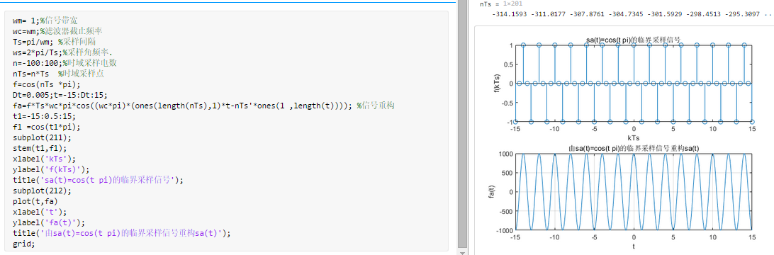
We select the signal \(f(t)=S a(t)\) as the sampled signal, which, when sampled at \(\omega_{s}=2 \omega_{m}\), is called pro
Boundary sampling. We take the ideal low-pass cutoff frequency \(\omega_{c}=\omega_{m}\) The following program implements the following for the signal \(f(t)=S a(t)\)
Sampling and reconstruction from that sampling signal recovery \(S a(t):\)
wm= 1;	%信号带宽
wc=wm;	%滤波器截止频率
Ts=pi/wm; 	%采样间隔
ws=2*pi/Ts;	%采样角频率.
n=-100:100;	%时域采样电数
nTs=n*Ts 	%时域采样点
f=sinc(nTs/pi);
Dt=0.005;t=-15:Dt:15;
fa=f*Ts*wc/pi*sinc((wc/pi)*(ones(length(nTs),1)*t-nTs'*ones(1 ,length())); %信号重构
t1=-15:0.5:15;
f1 =sinc(t1/pi);
subplot(211);
stem(t1,fl);
xlabel(kTs');
ylabel(f(kTs);
title('sa(t)=sinc(t/pi)的临界采样信号');
subplot(212);
plot(t,fa)
xlabel(t);
ylabel(fa(t);
title('由sa(t)=sinc(t/pi)的临界采样信号重构sa(t)');
grid;
Aliasing Reason
So far the case was discussed when no overlaps occur in the spectrum of the sampled signal. Hence when the upper frequency limit \(\omega_\text{u}\) of the real-valued low-pass signal is lower than \(\frac{\omega_\text{s}}{2}\). Here a perfect reconstruction of the continuous signal \(x(t)\) from its discrete counterpart \(x[k]\) is possible. However when this condition is not met, the repetitions of the spectrum of the continuous signal overlap. This is illustrated in the following
In this case no perfect reconstruction of the continuous signal by low-pass filtering (interpolation) of the sampled signal is possible. The spectrum within the pass-band of the low-pass contains additional contributions from the repeated spectrum of the continuous signal. These contributions are known as aliasing. It becomes evident from above discussion of ideal reconstruction that the amplitude values are reconstructed correctly at the time-instants \(k T\). However, in between these time-instants the reconstructed signal \(y(t)\) differs from the sampled signal \(x(t)\) if aliasing is present.
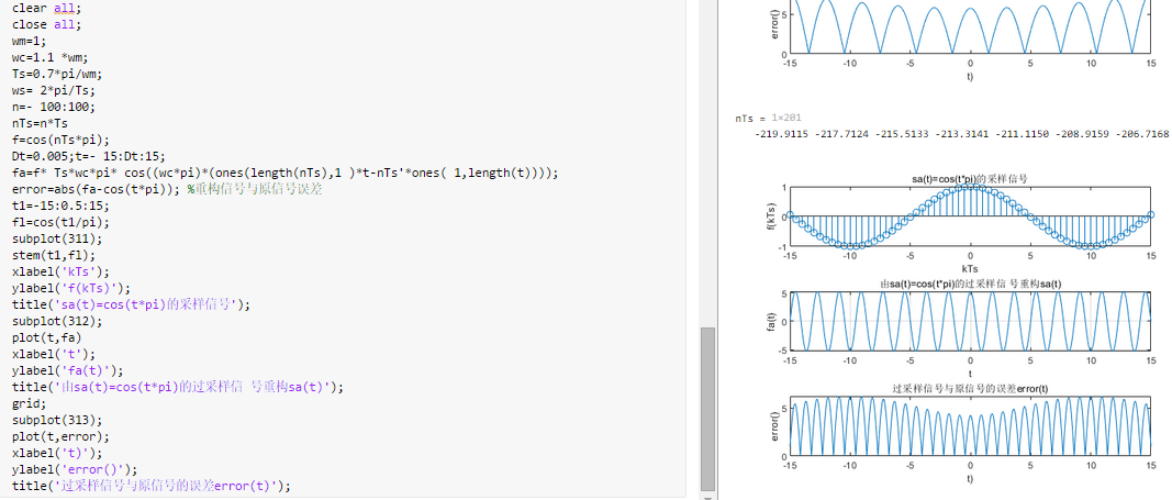
Implementation
wm=1;
wc=1.1 *wm;
Ts=0.7*pi/wm;
ws= 2*pi/Ts;
n=- 100:100;
nTs=n*Ts
f=sinc(nTs/pi);
Dt=0.005;t=- 15:Dt:15;
fa=f* Ts*wc/pi* sinc((wc/pi)*(ones(length(nTs),1 )*t-nTs'*ones( 1,length(t))));
error=abs(fa-sinc(t/pi)); %重构信号与原信号误差
t1=-15:0.5:15;
fl=sinc(t1/pi);
subplot(311);
stem(t1,fl);
xlabel('kTs');
ylabel('f(kTs)');
title('sa(t)=sinc(t/pi)的采样信号');
subplot(312);
plot(t,fa)
xlabel('t');
ylabel('fa(t)');
title('由sa(t)=sinc(t/pi)的过采样信号重构sa(t)');
grid;
subplot(313);
plot(t,error);
xlabel('t)');
ylabel('error()');
title('过采样信号与原信号的误差error(t)');
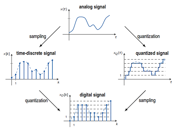
summary
!credit: bachelors module Signals and Systems, Communications Engineering, Universität Rostock.[email protected].
The order of sampling and quantization can be exchanged under the assumption that both are memoryless processes. Only digital signals can be handled by digital signal or general purpose processors. The sampling of signals is discussed as a first step towards a digital signal.