
文章目录[隐藏]
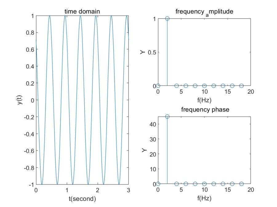
三角函数的时频图和复频图
clear;clf;
syms t;
f=2;T=1/f;t0=0;
A=1;
%ft=A*sin(2*pi*f*t);
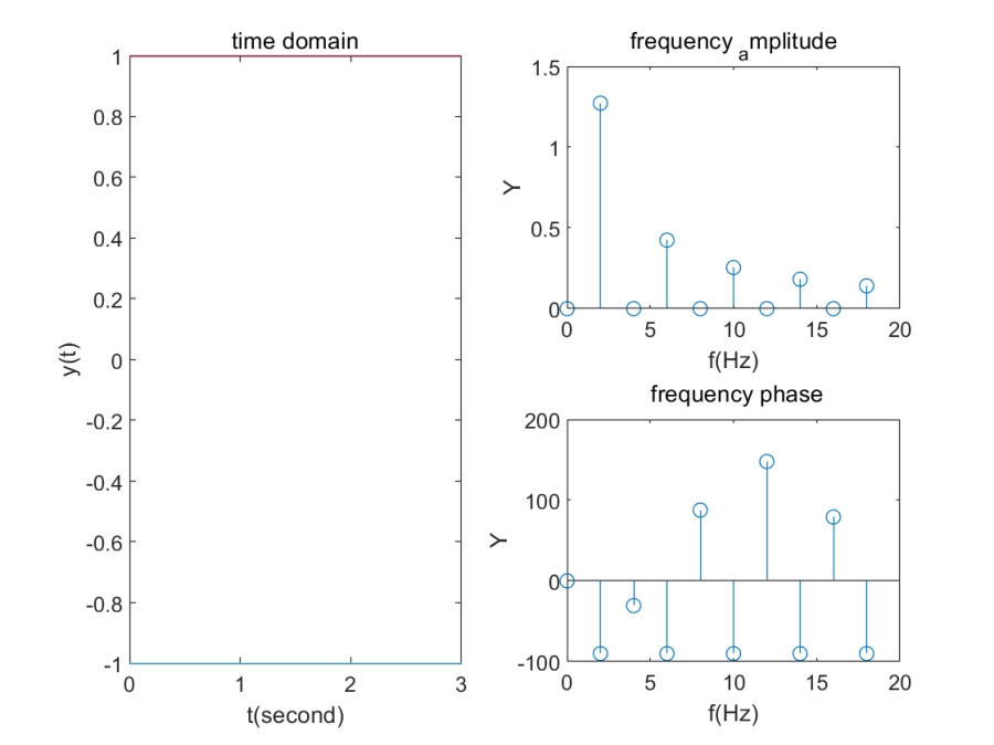
ft=A*cos(2*pi*f*t+pi/4);
subplot(2,2,[1,3]); fplot(ft,[0 3]);title("time domain" ); xlabel( 't(second)');ylabel( 'y(t)' );
w = 2*pi*f;N =10;
Fn = zeros(1,N);
Wn = zeros(1,N);
for k = 0:N-1
Fn(k+1) = 2*1/T*int(ft*exp(-1j*k*w*t),t, [t0, t0+T]);
Wn(k+1) = k*w;
end
subplot(2,2,2); stem(Wn/ (2*pi),abs(Fn));title('frequency_ _amplitude' ); xlabel('f(Hz)' );ylabel('Y');
subplot(2,2,4); stem(Wn/ (2*pi),angle(Fn)*180/pi);title(' frequency_ phase'); xlabel('f(Hz)' );ylabel('Y')
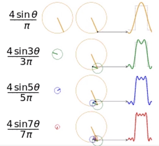
方波信号的时频图和复频图
实际上方波信号也是三角函数的加和,可以从复频图中看出。
clear;clf;
t=0:0.01:3;
f=2;T=1/f;t0=0;
A=1;
%ft=A*sin(2*pi*f*t);
ft=square(2*pi/T*t);
subplot(2,2,[1,3]); fplot(ft,[0 3]);title("time domain" ); xlabel( 't(second)');ylabel( 'y(t)' );
w = 2*pi*f;N =10;
Fn = zeros(1,N);
Wn = zeros(1,N);
for k = 0:N-1
  fun=@(t) square(2*pi/T*t).*exp(-1j*k*w*t);
  Fn(k+1) = 2/T*integral(fun,t0,t0+T);
  Wn(k+1) = k*w;
end
subplot(2,2,2); stem(Wn/ (2*pi),abs(Fn));title('frequency_ _amplitude' ); xlabel('f(Hz)' );ylabel('Y');
subplot(2,2,4); stem(Wn/ (2*pi),angle(Fn)*180/pi);title(' frequency_ phase'); xlabel('f(Hz)' );ylabel('Y')
信号转换可以找到信号的特性
clear;clf;
Fs = 1000;
ts = 1/Fs;
N = 3000;
t = (0:N-1)*ts;
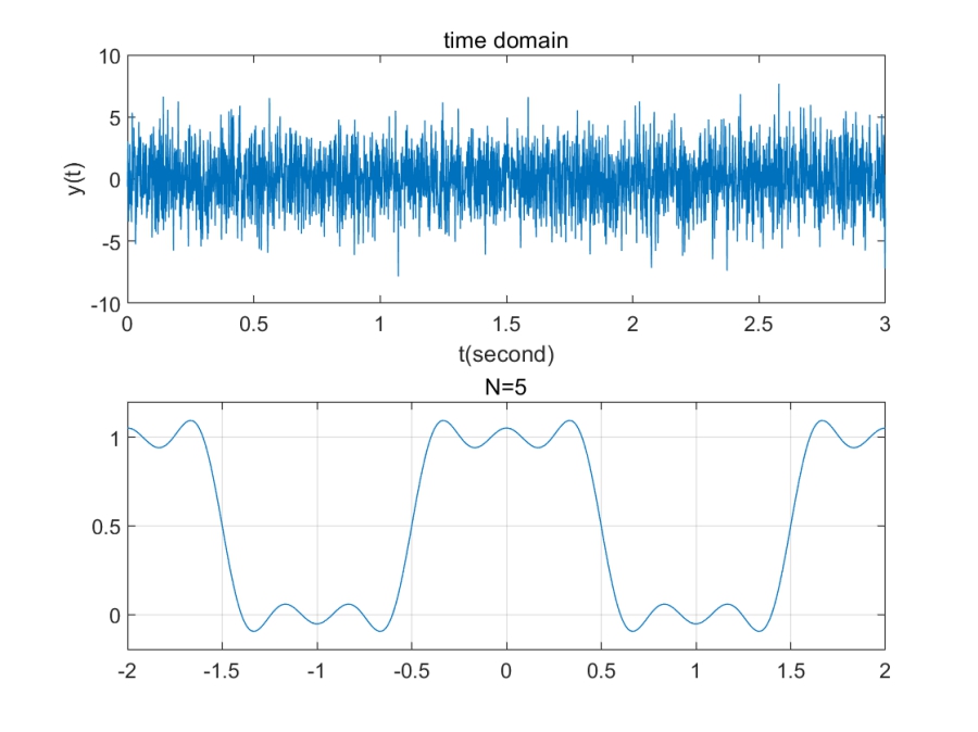
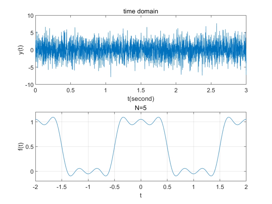
signal1 = 0.7*sin(2*pi*50*t)+sin(2*pi*120*t)+2*randn(size(t));
subplot(2,1,1);plot(t,signal1); title('time domain'); xlabel('t(second)');ylabel('y(t)');
Y = fft(signal1);
Y = abs(Y/N);
Y = Y(1:N/2+1);
Y(2:end) = 2*Y(2:end);
f = (0:N/2)*Fs/N;
subplot(2,1,2);plot(f,Y); title(' frequency domain' ); xlabel('f(Hz)');ylabel('Y');
 一种看时域图的角度
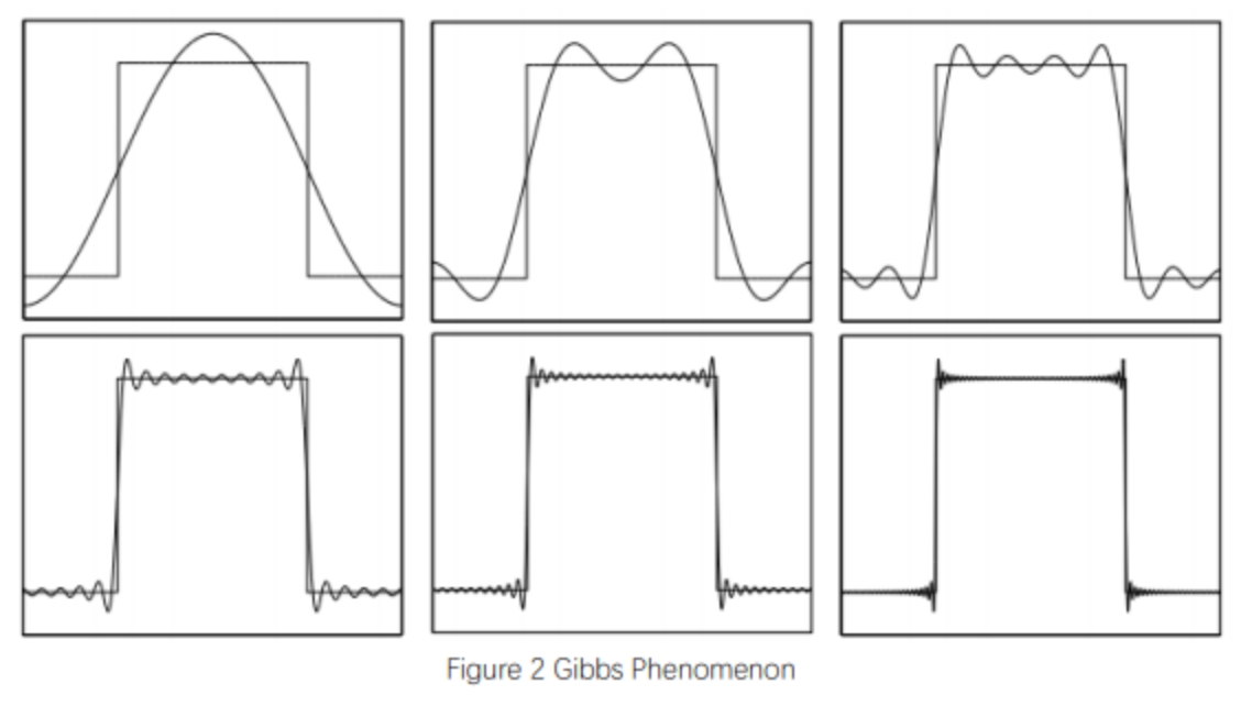
方波是一种频域三角函数
t = -2:0.001:2;
N = input('N=');
a0 = 0.5;
f = a0*ones(1,length(t));
for n=1:2:N
f = f+cos(n*pi*t)*sinc(n/2);
end
plot(t,f);grid on;
title(['N=' num2str(N)]);
xlabel('t');ylabel('f(t)');
axis([-2,2,-0.2,1.2])
t = -2:0.001:2;
N = input('N=');
T1 = 2;
w1 = 2*pi/T1;
fun = @(t) t.^0;
a0 = 1/T1*integral(fun,-0.5,0.5);
f = a0;
an = zeros(1,N);
bn = zeros(1,N);
for i = 1:N
fun = @(t) (t.^0).*cos(i*w1.*t);
an(i) = 2/T1.*integral(fun,-0.5,0.5);
fun = @(t) (t.^0).*sin(i*w1.*t);
bn(i) = 2/T1.*integral(fun,-0.5,0.5);
f = f + an(i)*cos(i*w1.*t)+bn(i)*sin(i*w1.*t);
end
plot(t,f); grid on;
title(['N=' num2str(N)]);
axis([-2 2 -0.2 1.2]);