

文章目录[隐藏]
Filters
category
低通(low-pass filter, LPF)
高通(high-pass filter, HPF)
带通(band-pass filter, BPF)
带止(band-stop filter, BSF)
We focus on low-pass filter, similar concepts and results hold for high-pass and band-pass filter.
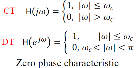
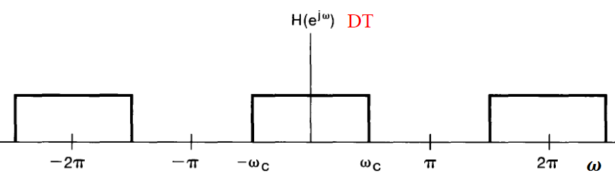
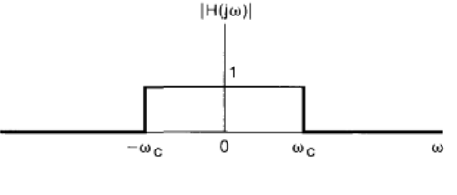
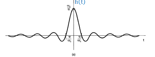
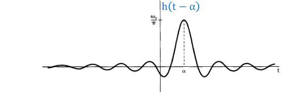
Ideal low-pass filter: zero phase
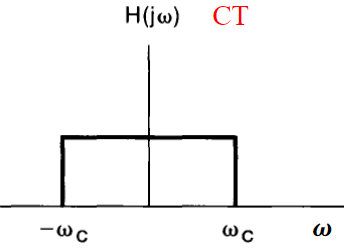
$$\begin{aligned}
h(t) &=\frac{1}{2 \pi} \int_{-\infty}{\infty} \mathrm{H}(j \omega) e{j \omega t} d \omega \
&=\frac{1}{2 \pi} \int_{-\omega_{c}}{\omega_{c}} 1 \cdot e{j \omega t} d \omega \
&=\left.\frac{1}{2 \pi} \cdot \frac{1}{j t} e^{j \omega t}\right|{-\omega{c}} ^{\omega_{c}} \
&=\frac{1}{2 \pi} \cdot \frac{1}{j t} \cdot 2 j \sin \left(\omega_{c} t\right) \
&=\frac{\sin \omega_{c} t}{\pi t}=\frac{\omega_{c}}{\pi} \operatorname{sinc}\left(\omega_{c} t\right) \
h(n) &=\frac{\sin \omega_{c} n}{\pi n}=\frac{\omega_{c}}{\pi} \operatorname{sinc}\left(\omega_{c} n\right)
\end{aligned}$$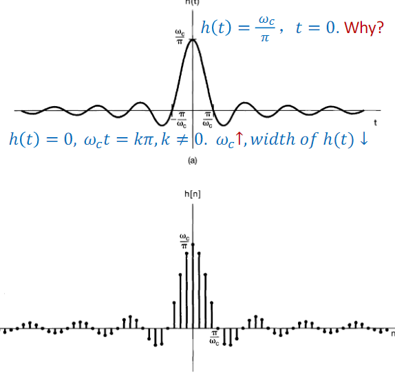
\(s(t)=\int_{-\infty}^{t} h(\tau) d \tau\) 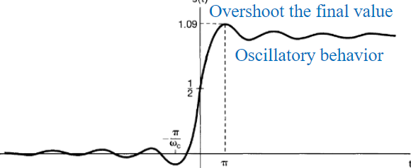
\(s(n)=\sum_{m=-\infty}^{n} h(m)\)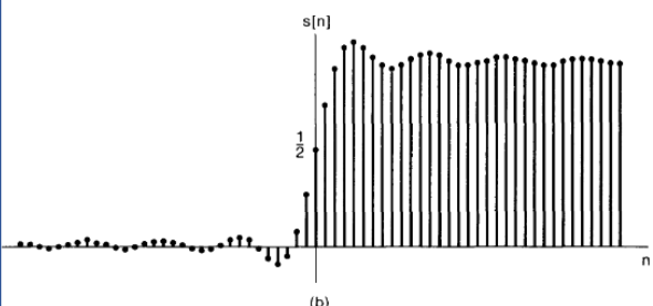
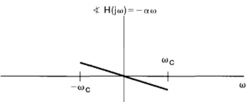
Ideal low-pass filter: linear phase
rotate for \(-\alpha \omega\)
Nonideal low-pass filter: frequencydomain
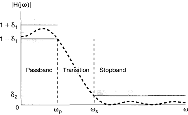
- Pass band: $0-\omega_{p}$, stop band: \(\omega>\omega_{s}\) transition: \(\omega_{s}-\omega_{p}\)
- Pass-band ripple: \(\delta_{1}\), stop-band ripple: \(\delta_{2}\)Linear (nearly) linear phase over the passband is desirable.
Nonideal low-pass filter: timedomain
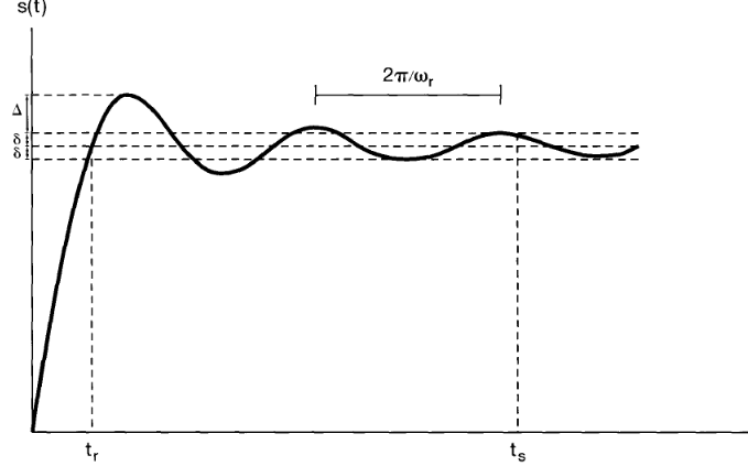
- Rise time: \(t_{r}\) overshoot: \(\Delta\)
- Ringing frequency: \(\omega_{r}\) settling time: \(t_{s}\)
e.g. Nonideal low-pass filter
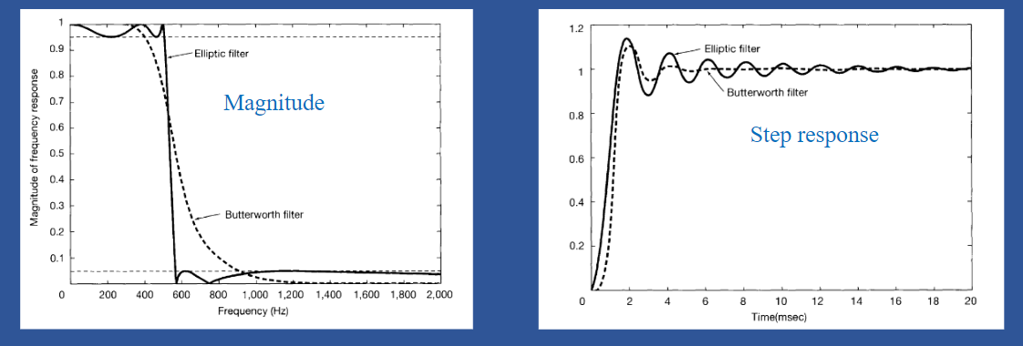
- Fifth-order Butterworth filter and a fifth-order elliptic filter
- Same cutoff frequency
- Same passband and stopband rippleThere's trade-off between time-domain characteristic \(t_{s}\) and fregurency domain characteristic \(\omega_{s}-\omega_{p}\)
Ideal vs. non-ideal filter
Gain.
- The ideal filter is fixed at a gain of 1 in the passband, which means that the input signal of the passband is "completely" passed, while the gain of the band is fixed at 0, which means that the input signal of the band is "completely" filtered out.
- The gain of a non-ideal filter is a function of frequency and not fixed.
Cut-off frequency.
- The ideal filter passband can be switched instantaneously between the stopband and the passband.
- The non-ideal filter cannot switch instantaneously between the passband and the stopband, its attenuation (gain) varies continuously with frequency, so there is a transition band, and the gain of the stopband cannot reach 0.
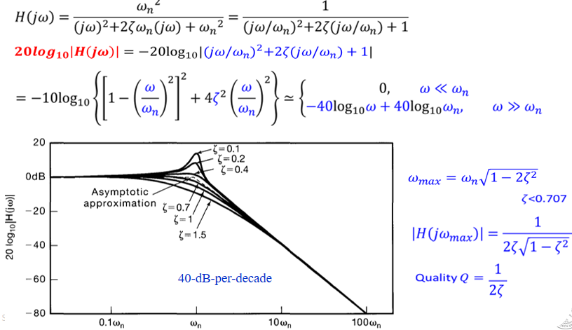
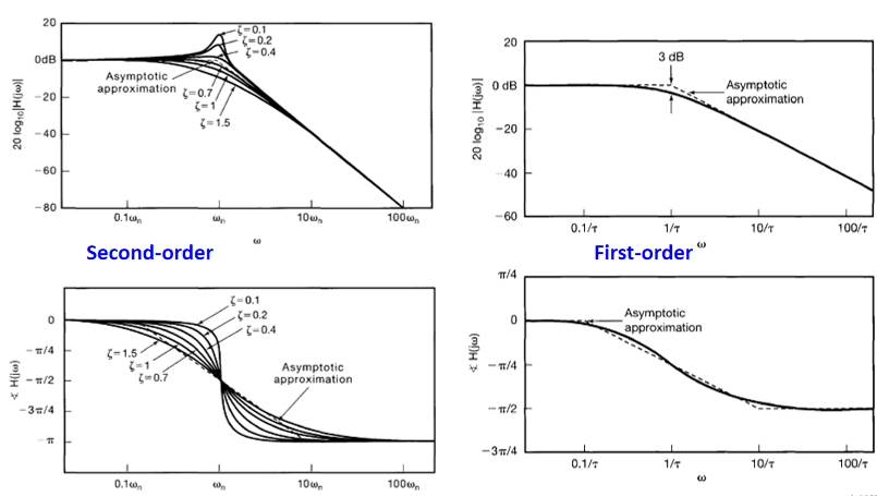
Bode Plot
The bode plot is for first and second-order CT system
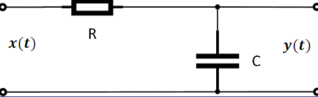
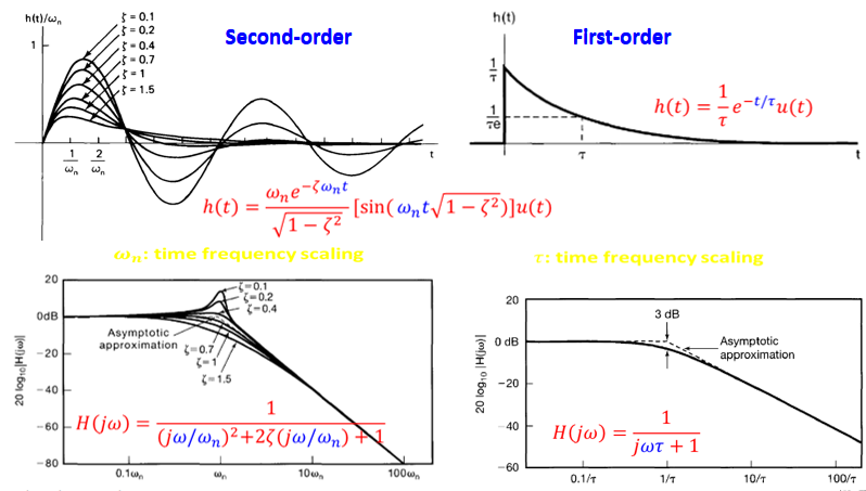
First-order CT system
$$\begin{aligned}
\text { Differential equation: } & C \frac{d y(t)}{d t}=\frac{x(t)-y(t)}{R} \
& \tau\left(\frac{d y(t)}{d t}\right)+y(t)=x(t), \tau=R C
\end{aligned}$$
$$\begin{aligned}
\text { Frequency response: } &\tau j \omega Y(j \omega)+Y(j \omega)=X(j \omega)\
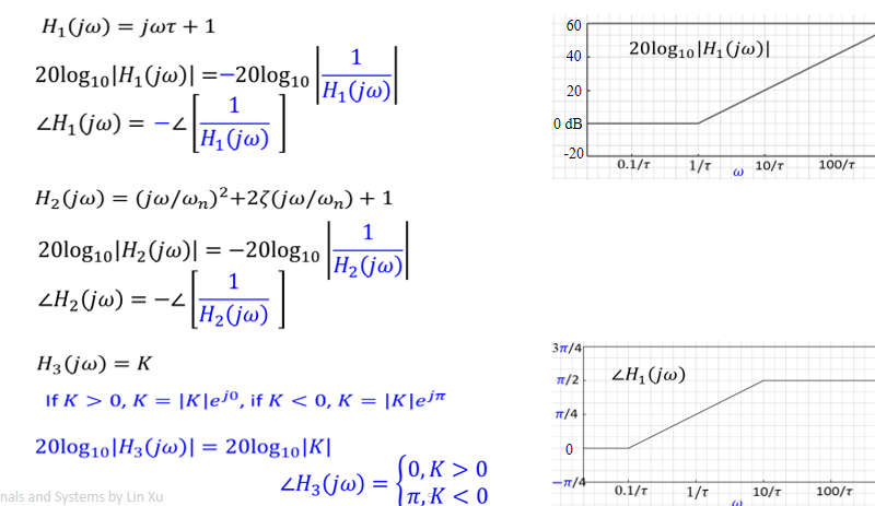
&H(j \omega)=\frac{Y(j \omega)}{X(j \omega)}=\frac{1}{\underbrace{(j \omega \tau)+1}}_{\text {First order }}
\end{aligned}$$
Basic deduction
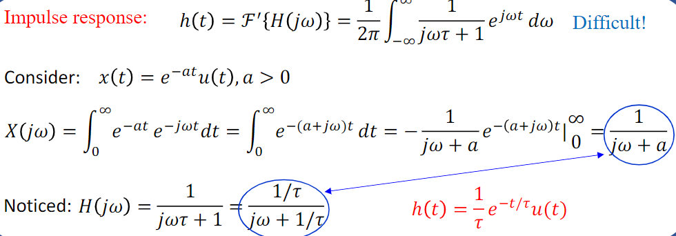
\(\tau:\) time constant
\(t=\tau, h(t)=1 /(\tau e)\)
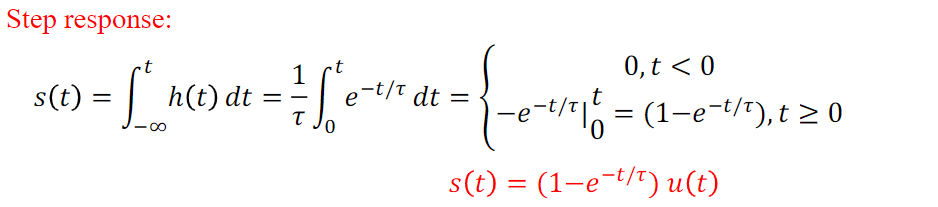
\(s(t)=1-1 / e\) 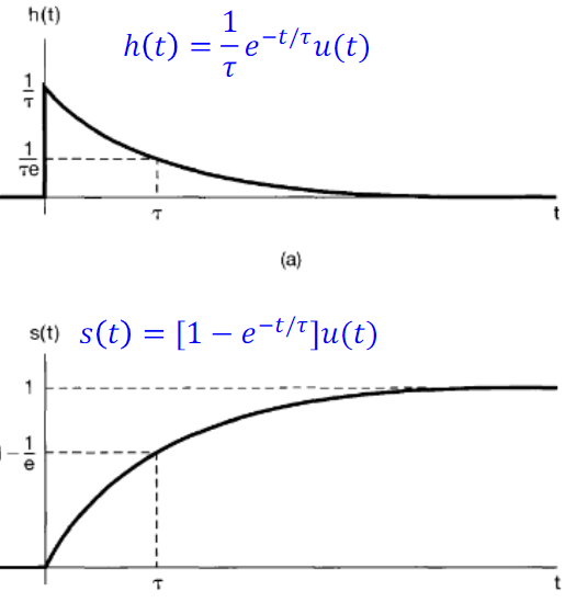
\(\tau \downarrow, h(t)\) decays more sharply
\(s(t)\) rises more sharply
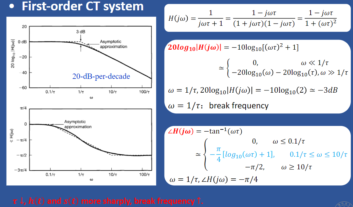
The reason why for the  is they be approximated by the domain by the \([\frac1{10\tau},\frac{10}\tau]\) to \(-\frac4\pi[log_{10}(\omega\tau)+1]\)
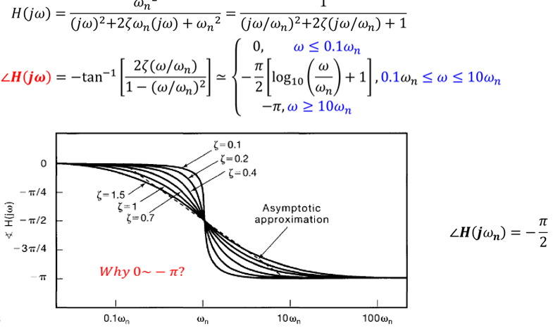
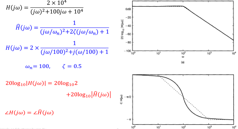
Second-order CT system: differential equation
physical meaning
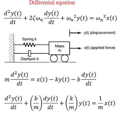
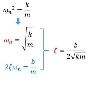
Frequency response \(\frac{d^{2} y(t)}{d t}+2 \zeta \omega_{n} \frac{d y(t)}{d t}+\omega_{n}^{2} y(t)=\omega_{n}^{2} x(t)\)
\begin{array}{l}j \omega)^{2} Y(j \omega)+2 \zeta \omega_{n}(j \omega) Y(j \omega)+\omega_{n}^{2} Y(j \omega)=\omega_{n}^{2} X(j \omega) \\ H(j \omega)=\frac{\omega_{n}^{2}}{(j \omega)^{2}+2 \zeta \omega_{n}(j \omega)+\omega_{n}^{2}}\notag\end{array}
\]
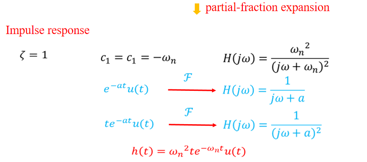
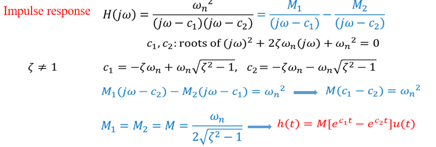
when \(\zeta>1\) the power is real, we can't apply Euler equation, just output the graph.
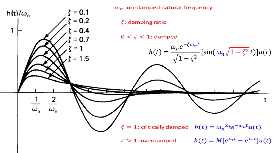
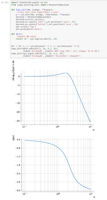
some param difference in Bode

implementation
Reference
- Lecture Notes on Signals and Systems by Sascha Spors.[email protected]
- signal_system_dsp Alan V. Oppenheim