[Parallel Computing] Loop dependence analysis

Intro

shared memory algorithm design

image-20200505182020225

For non-shared memory algorithms, we have to utilize bararrier to gain data transformed.

image-20200505182116133

for shared memory database algorithm, we have to decide the group part of the task that shared memory a lot . Then just apply the inserting directives of omp or mpi

Design considerations

two main considerations lies in data dependence and load balance so we have to apply the following steps

  • data dependence analysis
  • static r dynamic and block r cyclic work assignment
  • variable specification whether using shared private r reduction and row-wise r column-wise
    • shared variables cause cache coherence traffic and much lower performance
    • private and reduction variables don't need synchronization
    • dimension mapping is more relying on the cache locality

Main Consideration for data dependence analysis

RAW & WAR & WAW

all the collations should be avoided though they might run into right situations

Goal is to we should run all the dependent situation on the same processor.

loop dependence analysis

  • loop-carried dependence
    • dependence exists across different iterations of loop
  • loop-independent dependence
    • dependence exists within the same iteration of loop

example

image-20200505191450951

iteration-space traversal graph (ITG)

  • iteration-space traversal graph is a line graph showing the order of traversal in the iteration space.
  • image-20200505192641248

loop-carried dependence graph (LDG)

  • Given the ITG, can determine the dependence between different loops.
  • Loop-carried Dependence Graph (LDG) shows the loopcarried true/anti/output dependence relationships.
  • Node in LDG is a point in the iteration space.
  • Directed edge in LDG is the dependence.
  • LDG helps identify parts of the loop that can be done in parallel.

examples

image-20200505193459997
image-20200505193641884
image-20200505193657284
image-20200505194356931
image-20200505194556118


Distance and direction vector

image-20200505194745834
image-20200505195031615

Loop

image-20200505195226568
image-20200505195950287
image-20200505204740523
image-20200505204811678

Algorithm analysis

image-20200505205040713

Why you should use `express`

introduction

I manually do some stuff like

wget -r -p -np -k http://ics.nju.edu.cn/~jyywiki/

Many of the time you may get into the scenario the page you scripy from the website. they are rendered by the js. Admittedly, you can continue to use request_html. The idea is to use Chroium core to dynamically render the js page and grab the important information.

from requests_html import HTMLSession

If you want to deploy them locally, you have to get the express.

var express = require('express');
var path = require('path');
var ejs = require('ejs');
//import the package here

var app = express();

// view engine setup
app.set('views', path.join(__dirname, '/wiki'));
app.engine('html', require('ejs').__express);  
app.set('view engine', 'html');
//youcan implement the function used in the cache page here.
router.get('/*', function(req, res, next) {
  res.type('html');
  res.render('*');
});

//credit: https://blog.csdn.net/u011481543/article/details/79696565
node server.js

Save it to the server.js with the relative path and run

[Parallel Computing] SpMV

Intro

  • Sparse matrix vector multiplication.
  • Many scientific algorithms require multiplying a matrix by a vector.
    • Optimization (e.g. conjugate gradient low degree mesh.), iterative methods (solving linear systems), eigenvalue methods (e.g. graph partitioning vx), simulations (e.g. finite elements), data analysis (e.g. Pagerank the web connectivity matrix).
  • The matrices are often sparse.
    • In an nxn matrix, there are \(O(n^2)\) nonzero elements.

image-20200420095011605

image-20200420095335093

image-20200420095418927

DIA Format

image-20200420095439285

ELL format

image-20200420095732832

COO format

image-20200420095827947

CSR format

image-20200420095843518

image-20200420095942099

Hybird format

image-20200420100525622

what to use

image-20200420100455097

ELL kernel

image-20200420104856356

CSR scalar vector kernel

image-20200420104830242

CSR vector kernel

image-20200420104812194

COO vector kernel

image-20200420105358361

image-20200420104747538

[Parallel Computing] Concurrency bugs

  • In parallel system, high performance achieved by using algorithm with high parallelism, good load balancing, memory locality, etc.
  • But must also ensure multiple concurrent threads / processes operate correctly.
  • Concurrency bugs can arise due to unexpected interleaving of concurrent threads.
  • One of the most difficult issues to deal with in parallel / distributed computing.
    • Bugs occur at random times depending on the interleaving.
    • Bugs don’t occur during testing, but they will eventually occur in system deployed system.
    • Humans have hard time anticipating and resolving concurrency bugs.Concurrency bugs can have very serious consequences.

      Therac-25 radiation therapy system had a concurrency bug that led to radiation overdose and death of several patients.

      Space shuttle aborted 20 minutes before maiden launch due to concurrency bug in its avionics software.

eliminating concurrency bugs

  • Multiple ways, each with pros and cons.
  • Critical sections and locks
    • Prevent processes from accessing a block of code at the same time.
    • Easy to use, effective for some problems.
    • But cause contention, overhead and serialization.
    • Need to decide how much code to lock.
    • Too little, and may still get concurrency bug.
    • Too much, and we lose parallelism and performance.
  • If processes acquire several locks, they need to coordinate to maintain correctness, avoid deadlock.
  • Low priority that acquires a lock can delay high priority thread (priority inversion).
  • Despite these problems, locks are still the most widely used solution.
  • transactional memory
    • A block of code is defined as a transaction, i.e. the block of code either executes atomically or doesn’t execute at all.
    • Keep track of reads and writes done by a transaction. If two concurrent transactions read and write to same memory location, abort one of them, i.e. undo all the changes it made.
    • Two concurrent transactions accessing different memory locations can both commit, i.e. all the changes it made are made permanent.
    • Transactional memory can either be implemented in hardware (HTM) or software (STM).
    • HTM has limits of size and type of transactions it can handle. Implemented in e.g. Intel Haswell, IBM Power8.
    • STM is more flexible, but can be very slow.
  • Write your own concurrent code, without hardware support.
    • Challenging for most programmers. Not scalable in terms of productivity.
    • Correct, efficient algorithms are often research level publications.

Mutual exclution

  • Given n concurrent processes that want to perform a critical section (CS), mutual exclusion can satisfy the following properties.
    • No two processes are in CS at same time.
    • If several processes want to enter the CS, at least one succeeds in finite time (deadlock freedom).
    • If several processes want to enter the CS, every process succeeds in finite time (wait freedom).
  • All (useful) mutex algorithms satisfy first and second properties.
  • Some algorithms satisfy the third property, but have lower performance.

Mutual exclusion algorithms

  • Mutex is provided by locks. But how are locks implemented?
    • Depends on the type of operations the underlying hardware supports.
    • First type of algorithm uses only read / write operations.
    • Second type uses hardware synchronization primitives such as test-and- set (TAS) or compare-and-swap (CAS), provided in most processors.
  • TAS(x) tests if a Boolean variable x is true.
    • If x == false, it sets x to true.
    • Returns x’s value before the TS.
    • All these steps done atomically, without interruption from other threads.
    • getAndSet(x) is like TAS(x), but allows non-Boolean x.
  • CAS(x,v,v’) tests if variable x currently equals v. If so, it sets x to v’. Otherwise, it doesn’t change x. It also returns x’s current value.
    • Again, all this is atomic.
    • Algorithms also depend on a processor’s memory model.
    • Some processors reorder instructions to avoid stalls and obtain higher performance. This can break many lock algorithms.
    • Most lock algorithms assume memory model is sequentially consistent, i.e. the execution order of instructions from different processes is an interleaving of the instructions of each process in program order.

first attempt

  1. image-20200330212904433
  2. image-20200330223832949

[Parallel Computing] Shared Memory Programming and OpenMP

image-20200330122725049

shared memory model compared with mpi

  • Threads (e.g. Pthreads, Java)
    • individual sequences of instructions that can execute in parallel and access shared data
    • very general, because programmer have to manage everything.
  • parallel programming language/ library
    • a parallel language or library is used to create code
    • require new compiler
  • Compiler directives (OMP)
    • inserts compiler directives into a sequential program to specify parallelism and indicate shared data and the compiler translates into threads.
    • still uses threads underneath, but system manages the threads.
    • easy to program. but lose flexibility.

Processes and thread

  • Process(MPI)
    • separate program with its own variable, memory, stack and instruction pointer.
    • Different programs can't access each other's memory

    image-20200330123249520

  • thread(OMP)
    • Concurrent routine that shares the variables and memory space, but has its own stack and instruction pointer.

    image-20200330123330196

[Parallel Comuting] Cuda intrinsics

Reference: Cuda dev blog

why we introduce intrinsics

  • Race condition: Different outcomes depending on execution order.

  • Race conditions can occur in any concurrent system, including GPUs.

    • Code should print a =1,000,000.
    • But actually printed a = 88.
  • GPUs have atomic intrinsics for simple atomic operations.

  • Hard to implement general mutex in CUDA.

    • Codes using critical sections don’t perform well on GPUs anyway.

The atomic thread in critical section is not good in performance. The example is identified for variable d_aimage-20200415201026154

cuda atomics

Can perform atomics on global or shared memory variables.

  • int atomicInc(int *addr)
    • Reads value at addr, increments it, returns old value.
    • Hardware ensures all 3 instructions happen without interruption from any other thread.
  • int atomicAdd(int *addr, int val)
    • Reads value at addr, adds val to it, returns old value.
  • int atomicMax(int *addr, int val)
    • Reads value at addr, sets it to max of current value and val, returns old value.
  • int atomicExch(int *addr1, int val)
    • Sets val at addr to val, returns old value at val.
  • int atomicCAS(int *addr, old, new)
    • ā€œCompare and swapā€, a conditional atomic.
    • Reads value at addr. If value equals old, sets value to new. Else does nothing.
    • Indicates whether state changed, i.e. if your view is up to date.
    • Universal operation, i.e. can be used to perform any other kind of synchronization

examples

Finding max of array

image-20200415201746698
image-20200415201926626

improve it

we can improve it bu split the single global max into num_locals number of local max value.

Thread i atomically maxes with its local max. can max the local_max[locali],

image-20200415202001710

a better solution is to make it into the tree DS+CA

Compute the histogram

image-20200415202130295

! whether the data is stored on shared or global memory is depend on programmers

Shuffle intrinsics

! this intrinsic is not limited to cuda but all SIMD architecture

from avx256 vector elements we have

__m256 load_rotr(float *src)
{
#ifdef __AVX2__
    __m256 orig = _mm256_loadu_ps(src);
    __m256 rotated_right = _mm256_permutevar8x32_ps(orig, _mm256_set_epi32(0,7,6,5,4,3,2,1));
    return rotated_right;
#else
    __m256 shifted = _mm256_loadu_ps(src + 1);
    __m256 bcast = _mm256_set1_ps(*src);
    return _mm256_blend_ps(shifted, bcast, 0b10000000);
#endif
}

​

For Kepler architecture, we have 4 intrisics.

image-20200415225424500

The goal of the shuffle intrinsics is actually for optimizing Memory-Fetch Model

image-20200415230800174

butterfly operations

image-20200415223804087
image-20200415223136072

Assume we have at most shuffle instead of shared memory

image-20200415223508673
image-20200415223701215

[Parallel Computing] Amdahi and Gustafson, metrics to measure parallel program

2 great law

Amdahi

Amdahi law defines the speedup formula after the parallelization of the serial system.

The defination of the speedup: \(Speedup = \frac{Time\ before\ optimized} {Time\ after\ optimized}\). The higher the speedup, the better the optimization.

Proof: The time after optimization: \(T_nļ¼T_1(F+\frac1{n(1-F)})\), where \(T_1\) stands for the time before optimization, F is the percentage of serialized program,\((1-F)\) is the percentage of paralized program,n is the number of processor number. Take those into the equation we have \(\frac{T_1}{T_n}\),namely \(\frac{1}{(F + \frac{1}{n(1-F)})}\).

From the equation we can induce that the \(Speedup\) is inversely related with the \(F\). Also, from the equation, we can see that adding processor's number is just another method of providing \(Speedup\). Besides, lowering \(F\) can have the same effect.

For example in the \(ASC19\), besides merely applying the \(MPI\) parameter modification. The serialized part like initialization and special operation on the Qubits.

Gustafson

Gustafson is another important ways of evaluating the speedup rate

define the serialized processing time \(a\),parallelized processing time \(b\), namely single CPU situation, so the executing time \(a+b\) overall executing time \(a+nb,\) n denotes CPU number.

define the propertion F of a out of the executing time \(F=\frac{a}{(a+b)}\)

we get the final speedup rate. \(s(n)=a+\frac{nb}{a}+b=\frac a{a+b} + \frac{nb}{a+b} = F + \frac{n(b-a+a)}{a+b }= F + n(1-F)\)

From the equation, we have if the serialized part is tiny enough, $s(n)​ equals to the number of the CPU, so reducing the serialized part make sense, as well as adding the CPU core.

difference between two criteria

Two different law treats the parallel program from 2 different angles. Amdahi said that when the serial ratio is fixed, there is an upper limit by adding a CPU. By reducing the serial ratio and increasing the number of CPUs, the acceleration ratio can be improved. Gustafson is saying that when serial comparison tends to be very small, it can be seen from the formula that adding cpu can improve the speedup ratio

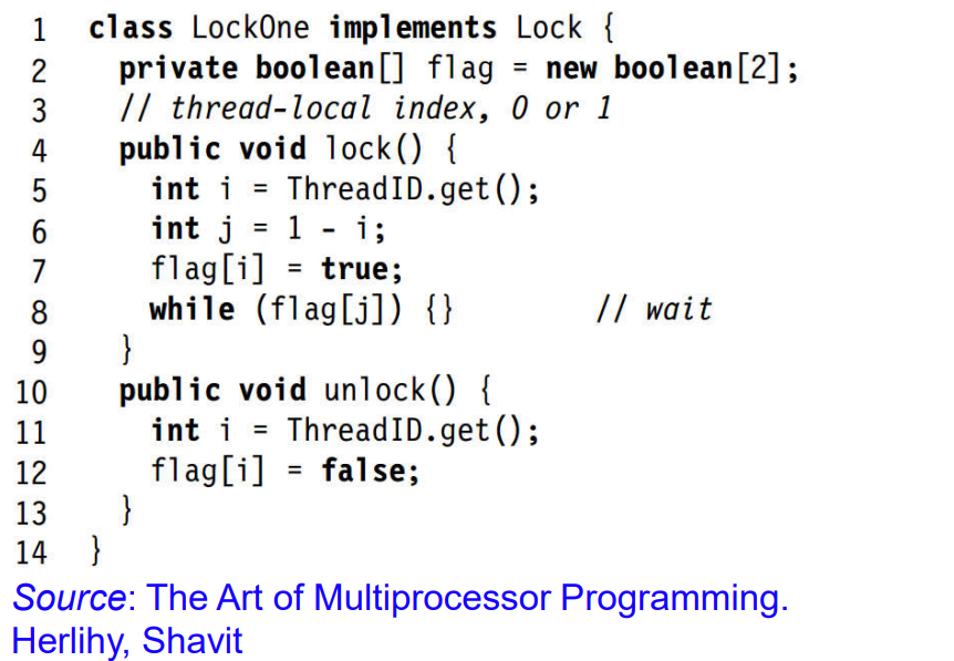
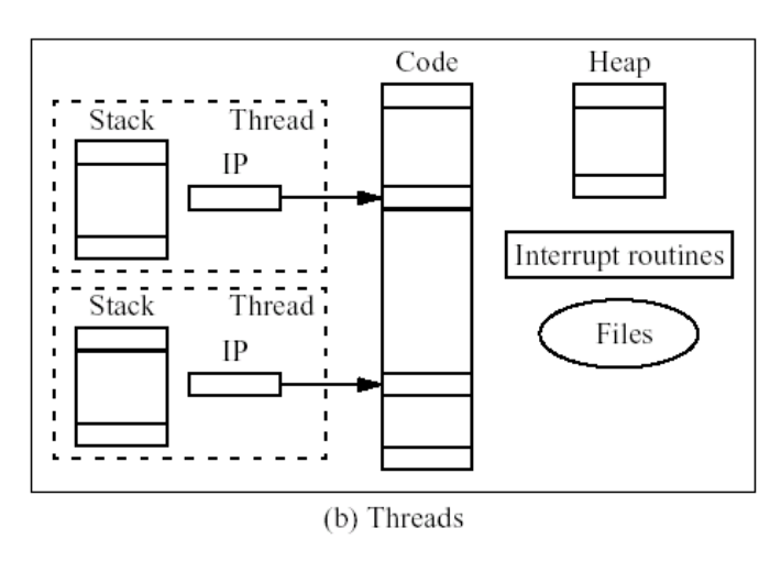
Multi-threaded features

Because of the inconsistency and security of data in a multi-threaded environment, some rule-based control is required. Java's memory model JMM regulates the effective and correct execution of multi-threading, and JMM is precisely the atomicity, visibility, and Orderly, so this blog introduces some multi-threaded atomicity, visibility and order.

Atomic

For single-threaded, it is indeed atomic, such as an int variable, change the value, it is the value when reading, this is very normal, we go to the system to run, it is also the same, because our operation Most of the system is 32-bit and 64-bit, int type 4 bytes, that is, 32-bit, but you can try the value of long type, long type is 8 bytes, which is 64-bit, if both threads Read and write it? In a multi-threaded environment, a thread changes the value of the long type and then reads it. The obtained value is not necessarily the value just changed, because your system may be 32-bit, and the long type is 64-bit. Yes, if both threads read and write to the long type, this will happen.

Visibility

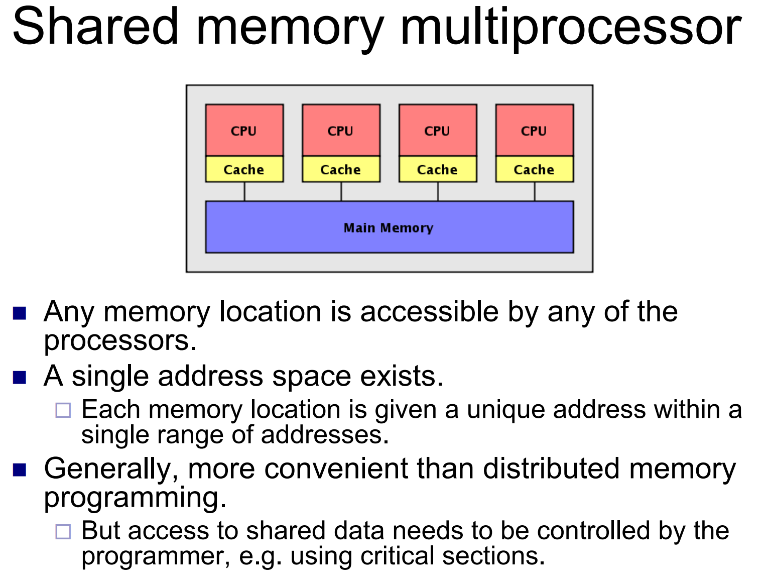
How to understand visibility? First of all, there is no visibility for single-threaded. Visibility is for multi-threaded. For example, if one thread has changed, does another thread know that the thread has changed, this is visibility . For example, the variable a is a shared variable. The variable a on cpu1 is cache optimized, and the variable a is placed in the cache. At this time, the thread on the other cpu2 changes the variable a. This operation is for cpu1. The thread is not visible, because cpu1 has been cached, so the thread on cpu1 reads the variable a from the cache, and found that the value read on cpu2 is not consistent.

Ordered

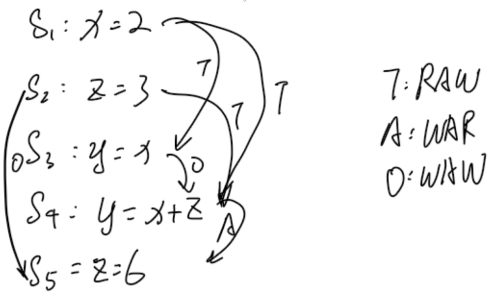
For single-threaded, the code execution of a thread is in order, which is true, but in a multi-threaded environment may not be necessary. Because in a multi-threaded environment instruction rearrangement may occur. In other words, in a multi-threaded environment, code execution is not necessarily ordered.

Since disorder is caused by rearrangement, then all instructions will be rearranged? of course not. The rearrangement follows: Happen-Before rule.
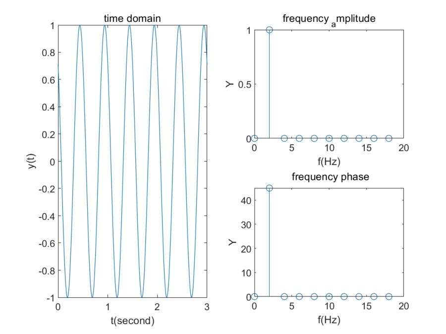
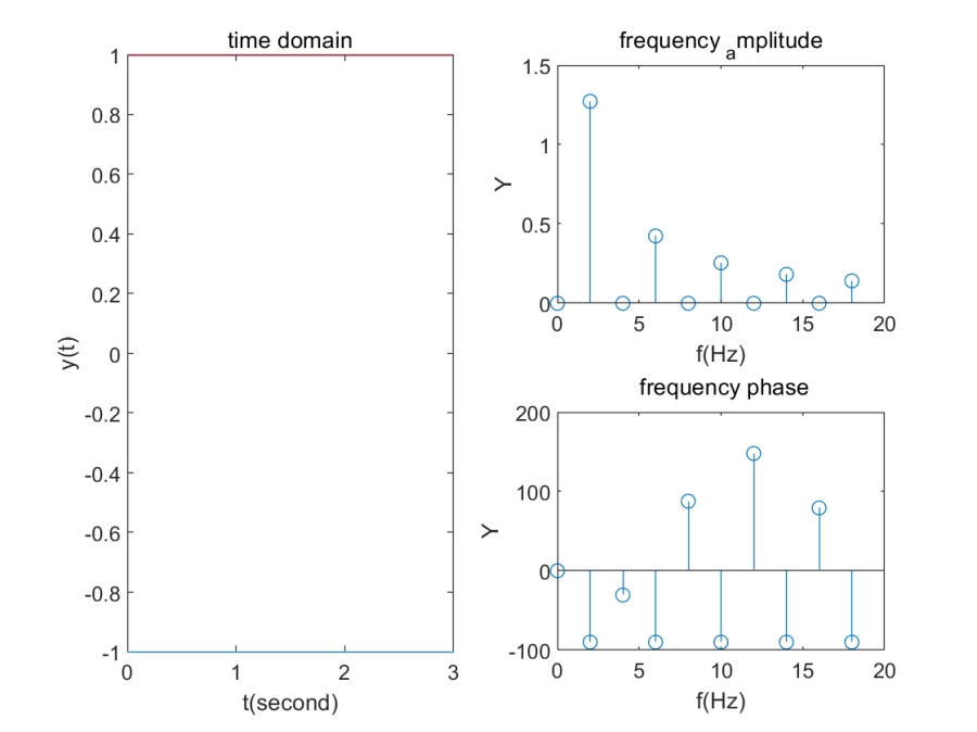
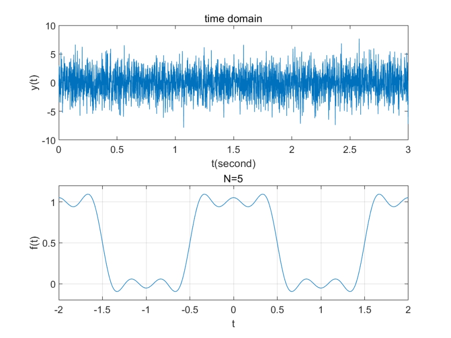
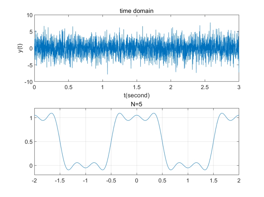
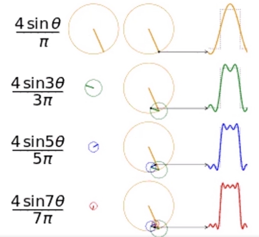
ęœ‰å…³é«˜č€ƒå‰ä½œę–‡ę˜Æå¦ę˜Æ'ę–‡é’å’Œę–‡é’č·Øę—¶ē©ŗåÆ¹čÆ'?

ä½™ä¹ƒäø€ä»‹č‰ę°‘ļ¼Œęœ€čæ‘č¦å†™ę–‡ē« ļ¼Œå›žé”¾ä»„å‰ēš„ę–‡ē« ļ¼Œęœ‰ę‰€ę„Ÿć€‚é«˜äø­ę—¶ęÆęÆå†™åŠä½œę–‡ę—¶ļ¼Œå¤§ę¦‚éƒ½ę·»åŠ äŗ†ęˆ‘åÆ¹å®¶åŗ­ļ¼Œęˆ‘åÆ¹ē¤¾ä¼šēš„ēœ‹ę³•ć€‚ęˆ‘å‡ŗē”ŸåœØäø€äøŖē§‘ęŠ€ć€ē†ę€§ļ¼Œäøé€åˆ©ć€ä»“å»Ŗå®žēš„å®¶åŗ­ć€‚å½“ę—¶ēš„čÆ­čØ€č”Øč¾¾éšåøøåøøčÆäøč¾¾ę„ć€‚ä½†å“ę˜Æę—¶č‡³ä»Šę—„ęˆ‘ēš„äŗŗē”Ÿå“²å­¦ć€‚

ę‰¾åˆ°ē—›č‹¦ēš„å¹øē¦

å‘Øå›½å¹³åœØå¤ę—¦åšäŗ†äø€åœŗć€Šē”Ÿę“»ēš„å¹øē¦ć€‹ę¼”č®²ļ¼Œåŗ§ę¬”äø€ä½å˜˜å£°ļ¼Œč‡ŖčÆ©č²Œē¾Žęœ‰ę‰ļ¼Œå®¶åŗ­ē¾Žå„½ļ¼Œęˆē»©ä¼˜å¼‚ļ¼Œå“ę— ę³•å¾—åˆ°å¹øē¦ć€‚

å¹øē¦äøę˜Æäø€ē§ę²”ęœ‰ē—›č‹¦ēš„ēŠ¶ę€ć€‚

ē”±äŗŽå½“ę—¶ęˆ‘ęŒŗå–œę¬¢čæ™å„čÆēš„ć€‚ęˆ‘č®ØåŽŒčæ™ē§ē§€ä¼˜č¶Šę„Ÿå“å®žé™…äøŠä»€ä¹ˆéƒ½äøč‡ŖēŸ„ēš„äŗŗļ¼Œä½†ęœ‰ę—¶å€™č‡Ŗå·±å“ę˜Æčæ™ę ·ēš„ć€‚ęˆ‘ę„Ÿęæ€ęˆ‘ēš„å®¶åŗ­ē»™ęˆ‘åø¦ę„ēš„č§†é‡Žć€é«˜åŗ¦ć€‚čæ™ä½æå¾—å½“ę—¶ęˆ‘åÆ¹å¾ˆå¤šā€œę–‡é’ā€å—¤ä¹‹ä»„é¼»ć€‚ę— ę‰€é€‚ä»Žåˆ°ęƒ³åÆ¹ä»–ä»¬å£čÆ›ē¬”ä¼ć€‚ęˆ‘å°‘äŗ†äø€ē§č£…é€¼ēš„ęƒ³ę³•ļ¼ŒåŒę—¶ęœ‰äŗ›č‡Ŗå‘ļ¼Œå› äøŗęˆ‘ęˆē»©å°±ę˜Æäøå¦‚åŒē­åŒå­¦ļ¼Œę— č®ŗęˆ‘å¤šä¹ˆåŠŖåŠ›ć€‚ä¹Ÿč®øę˜Æčƒ½åŠ›äøå¤Ÿå§ļ¼Œęˆ–č€…ęƒ³č¦ēš„å¤Ŗå¤šć€‚ę‰€ä»„ęˆ‘å†…åæƒčæ˜ę˜Æéžåøøč‡Ŗå‘ēš„ļ¼Œęƒ³é€ščæ‡ā€œēœ‹äøäøŠåˆ«äŗŗā€ļ¼Œę„å¾—åˆ°č‡Ŗčŗ«ēš„ę…°č—‰ć€‚

ęˆ‘åÆ¹čæ™ēÆ‡ę–‡ē« å¤§ä½“ēš„ęƒ³ę³•ę˜Æęƒ³å†™ęˆäøŽč‡Ŗå·±ēš„åÆ¹čÆć€‚å¦‚ęžœč‡Ŗå·±å·²ē»ę„Ÿå—åˆ°äø–äæ—ę„ä¹‰äøŠēš„å¹øē¦äŗ†ļ¼Œę˜Æå¦åŗ”čÆ„ēšˆä¾ē—›č‹¦ļ¼Œå†ä»Žē—›č‹¦äø­åÆ»ę‰¾č‡Ŗęˆ‘ēš„ä»·å€¼ć€‚

å‘Øå›½å¹³čæ™å„čÆå®žé™…äøŠä¹Ÿę˜Æäø€ē§ę”¾å¤§ę€§ēš„č§£čÆ»ć€‚ē—›č‹¦äøę˜Æå¹øē¦ēš„åÆ¹ē«‹é¢ć€‚ęˆ–č®øęœ‰ę—¶å€™čæ›å…„ē—›č‹¦ä¹Ÿčƒ½å¾—åˆ°å¹øē¦ļ¼Œäøē—›č‹¦ä¹ŸåÆä»„å¹øē¦ć€‚čæ™åÆ¹å¾ˆå¤šę–‡é’ę„čÆ“å°±ę˜Æä»–ä»¬ēš„å‘ęŒ„ē©ŗé—“äŗ†ć€‚ęÆ”å¦‚čæ™ē§ē—›č‹¦åÆä»„ę˜Æę‰¾åÆ»č„æē»Ŗē¦ę–Æčˆ¬ēš„ā€œęœ‰ē—›č‹¦å“å¾ˆå¹øē¦ā€ļ¼Œęœ€ē»ˆę‰¾åˆ°ē—›č‹¦ä¹Ÿå¾ˆå¹øē¦ć€‚ē„¶åŽå†č¾…ä»„åŽäø½ēš„äøŽčÆ„å·č€åøˆä¼šåæƒēš„ęƒ³ę³•ć€‚ä¾æåÆä»„å¾—åˆ°äøé”™ēš„åˆ†ę•°ć€‚

å½“ę—¶ęˆ‘åˆšä»Žä¼Æå…‹åˆ©å›žę„ę²”å¤šä¹…ļ¼Œę˜Æäø€ę¬”é«˜äŗŒäøŠēš„ęœˆč€ƒć€‚åŒę—¶ęŽ„č§¦å¾ˆå¤šå®¶é‡Œęœ‰é’±ļ¼ŒåŒę—¶åˆå¾ˆä¼˜ē§€ļ¼Œęœ€åŽäøä¹ē”³äøŠä¼Æå…‹åˆ©č®”ē®—ęœŗēš„äø€äŗ›åŒå­¦ļ¼Œčæ™ē§äŗŗēš„äŗŗē‰©č‚–åƒå°±ę˜Æå£äøŠčÆ“ēš„éƒ½ę˜Æę»”ę»”ēš„čµ„ęŗć€‚ę‰€ä»„ęˆ‘å°†čæ™ä½åŒå­¦åø¦å…„äŗ†ä»–ä»¬ć€‚ä»–ä»¬å…¶å®žå¾ˆå¹øē¦ļ¼ŒåÆä»„äø€å¤©ę¢äø€äøŖå„³å‹ć€‚ęƒ³č±”ēŽ‹ę€čŖć€‚ęˆ‘å¼€å§‹äŗ†ęˆ‘ēš„éŖ‚ęˆ˜ć€‚ęˆ‘åŒę—¶čæ˜ęƒ³åˆ°äŗ†å½“ę—¶ēš„ā€œčˆŖęÆā€ļ¼Œå³é€ščæ‡ęÆå¤©ē½‘äøŠå­¦ä¹ å­¦åˆ°3ē‚¹ēš„å„³ē”Ÿļ¼Œęœ€åŽč€ƒäøŠäŗ†ęø…åŽę–°äŗšä¹¦é™¢ć€‚ęˆ‘čÆ“ļ¼Œäøč¦é‚£ä¹ˆäøŗäŗ†å¹øē¦č€Œē—›č‹¦ć€‚čæ˜ęœ‰å°±ę˜Æęˆ‘ēš„äøä½œäøŗēš„ęÆäŗ²å’Œäøä½œäøŗēš„čÆ­ę–‡č€åøˆć€‚č‹„ę˜ÆęÆäŗ²ē»™åŠ›äø€ē‚¹ć€‚č‹„ę˜ÆčÆ­ę–‡č€åøˆē»™åŠ›äø€ē‚¹ć€‚ęˆ‘ä¼šå„½čµ°äø€ē‚¹ć€‚

ęˆ‘å¼•ē»ę®å…øļ¼Œå‘ŠčÆ‰ä»–ä»¬ę‰€č°“ēš„ā€œå°ęœ‰ęˆå°±ā€åœØę˜Žęø…ę—¶ēš„å¤œčˆŖčˆ¹äøŠå°±ęœ‰å¾ˆå¤šč‡Ŗå¹č‡Ŗę“‚ęœ€åŽč½å¾—č‡Ŗå·±ā€œäø€ę— ę‰€ēŸ„ā€ēš„äø‹åœŗć€‚å¾—åˆ°å››ä¹¦äŗ”ē»ēš„ēœŸä¼ åˆå¦‚ä½•ļ¼Ÿčæ™ē§å°†å…«č‚”å„‰äøŗåœ­č‡¬ļ¼Œé™·äŗŽč‡Ŗå·±ēš„čˆ’é€‚åŒŗēš„äŗŗļ¼Œå®žåˆ™ä»…å¾—åˆ°å­”å­ŸēØ‹ęœ±ēš„č¾¹č§’ę–™ļ¼Œé—¹å¾—åŖä¼šåÆ¹åÆ¹č”čæ™ē§ę¶äæ—ę–‡é’ę“ä½œć€‚ę²”ęœ‰ēœŸę­£ę„ä¹‰äøŠēš„åˆ›ę–° ļ¼Œä¹Ÿå³ę˜ÆęŠŠč‡Ŗå·±ę”¾åœØčˆ’é€‚åŒŗēš„ē»“ęžœć€‚å½“ę—¶ēš„äø­å›½ę²”ęœ‰čæ›ę­„ļ¼Œäŗŗå‡ē”Ÿäŗ§äø€ē›“ē»“ęŒåœØä½Žē‚¹åƒå¹“ēš„åŽŸå› čŽ«čæ‡äŗŽę­¤ć€‚ęˆ‘ä»¬ę”¾å¼ƒäŗ†ā€œē§‘ęŠ€ā€ļ¼Œč€Œę²‰ęµøäŗŽå¤äŗŗēš„č¾‰ē…Œć€‚

äŗŗéœ€č¦ē—›č‹¦ļ¼Œéœ€č¦ē—›č‹¦åŽ»åœ†ę»”å……å®žäŗŗē”Ÿļ¼Œä»Žč€Œé€ ē¦ē¤¾ä¼šć€‚

ęˆ‘ęƒ³čÆ“ļ¼Œäŗŗę˜Æč¦ęœ‰å®¶å›½ęƒ…ę€€ēš„ć€‚ę‚Øé‚£äŗ›å¹øē¦äøčæ‡ę˜Æå±ę°‘ęƒ³ēš„å±äŗ‹ć€‚ä»“å»Ŗå®žåˆ™éœ€å…³ę³Øę°‘ē”Ÿļ¼Œč‡Ŗå·±ē—›č‹¦ļ¼Œč°‹ę±‚å…Øē¤¾ä¼šēš„å¹øē¦ć€‚

äø€äøŖčŖę˜Žäŗŗęœ€å®¹ę˜“ęƒ³å®Œäŗŗē”Ÿļ¼Œę„Ÿč§‰äŗŗē”Ÿå°±é‚£ę ·ļ¼Œåšå„½åˆ†å†…ä¹‹äŗ‹ļ¼Œä½•åæ…ē—›č‹¦å‘¢ļ¼ŸäŗŽę˜ÆęÆå¤©ę‹˜ę³„äŗŽč‡Ŗå·±ēš„å°ē”®å¹øäø­ļ¼Œå¦‚ā€œé¾™åŗ”å°ā€ä¹‹ęµļ¼Œčæ™ę˜Æā€œå¹³åŗøä¹‹ę¶ā€ć€‚é‚£ä½å­¦ē”Ÿåŗ”ęŠŠč‡Ŗå·±ēš„ę‰€č°“ēš„č“¢åŠ›ęŠ•å…„č‡Ŗå·±ēš„ā€œē—›č‹¦ā€ļ¼Œčµ°å‡ŗčˆ’é€‚åœˆć€‚č€Œäøåŗ”åƒå„’å£«äø€ę ·ę²”ęœ‰ēœ¼å…‰ć€‚å®ƒå› č½¬åŒ–äøŗåŠ›é‡ļ¼Œé€ ē¦äŗŗē±»ć€‚

äø¤äøŖä¾‹å­ļ¼Œäø€ę­£äø€åć€‚å¤å·“é“¶č”Œč”Œé•æåˆ‡ę ¼ē“¦ę‹‰å’Œå‚»é€¼ēŽ‹ę€čŖć€‚

ē‚®č½°ę²”ęœ‰å¹øē¦ēš„äŗŗļ¼Œę²”ęœ‰ē—›č‹¦ēš„äŗŗć€‚

ā€œäŗŗéœ€åÆ»å¾—ę‰€ēˆ±ć€‚ā€ä¹”åø®äø»ē”Øčæ™å„čÆē»“ęŸē»™ā€œäø–ē•Œå¤§č„‘ā€ä»¬ēš„ę¼”č®²ļ¼Œę„åœØčÆ“ę˜Žäŗŗę€»čƒ½ę‰¾åˆ°å±žäŗŽč‡Ŗå·±ēš„ä»·å€¼ļ¼Œäøŗä¹‹ē—›ļ¼Œäøŗä¹‹ä¹ć€‚čæ™ä»½ē—›ę˜Æåø¦ęœ‰äø»č§‚åˆ¤ę–­ēš„ć€‚äøčƒ½éŗ»ęœØē›²ä»Žåœ°ē—›č‹¦äø‹åŽ»ļ¼ŒęŠ˜ē£Øč‡Ŗå·±å¾ˆē®€å•ļ¼Œä½†ē»äøčƒ½é™·å…„ēäŗ‹ēš„ē—›č‹¦ļ¼Œäøčƒ½č®©ē‰‡é¢åŗøäæ—ēš„ē—›č‹¦ęˆäøŗęˆå°±é«˜ę°“å¹³å¹øē¦ēš„ē»Šč„šēŸ³ć€‚å²é“ē”Ÿäø€ē”Ÿā€œåŸ‹ę²”ā€åœØē—…ē—›ē—›č‹¦ēš„ęžč‡“äø­ļ¼Œå“åœØåœ°å›å…¬å›­äø­ē»™å…Øäø­å›½äŗŗę°‘åœØę–‡é©åŽä»„ē”Ÿå‘½ę„ä¹‰ēš„ę…°č—‰ć€‚č‹č½¼ęˆé•æä¹‹č·Æäø–äŗŗēš†ēŸ„ļ¼Œä»Žé’å¹“åˆ°č€å¹“ēš„č·ƒå˜ļ¼Œä»Žę— ę³•ę‘†č„±åÆ¹ę—¶å¼Šēš„ęŸē¼šåˆ°ę— ä»„ä¼¦ęÆ”ēš„čƒøč„Ÿć€‚ä»–ēŖē “äŗ†č‹¦ēš„č¾¹ē•Œļ¼Œäøŗē™¾å§“ē–¾č‹¦å…±čˆžć€‚ä»–ēš„å¹øę˜Æ č‹¦å åŠ ēš„ē»“ęžœć€‚ē›øåäø‡åŽ†ęœ±ēæŠé’§å€’åœØäŗ†č‡£å­é˜“é˜³åˆ©ē›Šę–—äŗ‰ēš„č”€ę³Šå’Œäø‰å¾é«˜äø½ēš„ē—›č‹¦äø­ļ¼Œå¤±äŗ†åæƒę™ŗļ¼ŒęœŖčƒ½ē»­å¤§ę˜Žä¹‹å¹øļ¼Œå¼ å±…ę­£ä¹‹ę‰˜ļ¼Œē»ˆäŗ«å…¶ä¹ć€‚

ęˆ‘čæ™ę®µčÆęƒ³čÆ“ēš„å°±ę˜Æęœ‰ę„ä¹‰ēš„é«˜å±‚ę¬”ē—›č‹¦čƒ½åø¦ę„ę›“é«˜å±‚é¢ēš„å¹øē¦ć€‚

ę‰¾åˆ°ē—›č‹¦åŽēš„å¹øē¦ļ¼Œę˜Æäø€ē§ē£Øē ŗļ¼Œę›“ę˜Æäø€ē§čœ•å˜ć€‚äŗŗäøčƒ½ē®€å•ę»”č¶³ēŽ°ęœ‰ēš„ę”ä»¶ļ¼Œč€Œę›“åŗ”ęƒ³ē€å¦‚ä½•č½¬åŒ–ę”ä»¶äøŗę›“é«˜å±‚é¢ēš„å¹øē¦ć€‚é«˜å±‚ę¬”ēš„å¹øē¦å°±ę˜Æå®¶å›½ä¹‹å¹øć€‚åŒę—¶ļ¼Œå¹øē¦äøę˜Æē®€å•ē›²ē›®ēš„ļ¼Œč€Œę˜Æč¦ęœ‰åˆ¤ę–­äøŽå–čˆć€‚

ęˆ‘ēš„äŗŗē”Ÿå“²å­¦å°½å¦‚ę­¤ć€‚ä»Žäøę–­ēš„ē—›č‹¦å’Œę‰“å‡»ä¹‹äø‹åŽ†ē»ƒč‡Ŗå·±ć€‚ęˆ‘č¦å­¦ęŠ€ęœÆļ¼Œä¼šē®”äŗŗć€‚ęœ‰č‡Ŗäæ”ć€‚ęŠŠā€œå®¶å›½ä¹‹å¹øā€ä½œäøŗå·±ä»»ļ¼Œäæ®čŗ«é½å®¶ę²»å›½å¹³å¤©äø‹ć€‚ęˆ‘äøä¼šåšęˆ‘ēœ¼äø­ēš„å°äŗŗļ¼Œęˆ‘å¦ˆļ¼Œęˆ‘ēš„é«˜äø­čÆ­ę–‡č€åøˆļ¼Œliujingwenļ¼Œčæ˜ęœ‰é‚£åø®ē•™å­¦ē”Ÿä»¬ć€‚ęˆ‘ä¼šäøŗč‡Ŗå·±ēš„ę„ä¹‰å„‹ę–—ē»ˆčŗ«ļ¼Œäøŗē„–å›½å„åŗ·å·„ä½œ50幓。

čÆ“čÆ“čæ™ēÆ‡ę–‡ē« äøŗå•„ę˜Æäø‰ē±»äø‹å·ļ¼Œå³å¾—äŗ†44/70. å¤§č‡“äøŠę˜Æåé¢˜äŗ†ļ¼Œč€Œäø”ē”ØčÆęœ“ē“ ļ¼Œę²”å•„ę–™ć€‚å„½åƒč€åøˆēœ‹äøŠåŽ»ę²”ęœ‰åŒę„Ÿļ¼Œęˆ–č€…čÆ“ę ¹ęœ¬ę‡’å¾—čÆ»ć€‚čæ˜ęœ‰ļ¼Œå‘Øå›½å¹³åœØå“Ŗé‡Œļ¼Ÿ

čæ™ę˜Æäø€äøŖ17å²ēš„å°‘å¹“åœØä»…å‰©30åˆ†é’Ÿå®Œå·ēš„å†…åæƒē‹¬ē™½ć€‚ęˆ‘äøé€‚åˆč¢«åŠØēš„å­¦ä¹ ć€‚ä»Žčæ™ä»„åŽęˆ‘éƒ½ę˜Æå¾ˆäø»åŠØēš„ļ¼Œä»Žęœ¬č¢«ēˆ¶ęÆę‹‰ē€å‡ŗå›½ļ¼ˆęˆ‘č®¤äøŗę˜Æäø€äøŖå›é€ƒč€…ļ¼‰ļ¼Œåˆ°ä½œäøŗäø€äøŖåˆę ¼ēš„é«˜č€ƒē”Ÿć€‚ęˆ‘ęˆ–č®øåœØå½“ę—¶å°±åŗ”čÆ„č®¤čÆ†åˆ°å·®č·ļ¼ŒåÆęˆ‘č¢«č‡Ŗå·±å¤–č”Øč‡Ŗå¤§ļ¼Œå†…åæƒč‡Ŗå‘ēš„ę€§ę ¼ę‰€éŗ»ē—¹ļ¼Œč®¤äøŗē»čæ‡åŠŖåŠ›ļ¼Œäø€å®ščƒ½å¾—åˆ°å±žäŗŽęˆ‘ēš„äø€ē‰‡å¤©åœ°ć€‚åÆäŗ‹å®žę˜Æļ¼ŒčÆ­ę–‡č€åøˆäøē†č§£ęˆ‘ēš„åæƒę€ć€‚

ęˆ‘ęŒŗå–œę¬¢čÆ»å½“ę—¶ēš„é‚£äŗ›ę–‡é’ēš„ļ¼ŒēŽ°åœØä¼°č®”č½¬åø‚åœŗļ¼Ÿå­¦ę³•å¾‹ļ¼ŸęŠ‘ęˆ–å­¦ē»ęµŽäŗ†ć€‚ęˆ‘äŗŗåÆ¹ä»–ä»¬å—¤ä¹‹ä»„é¼»ć€‚ęˆ‘č®¤äøŗé‚£äøŖę—¶å€™ēš„ä½œę–‡ļ¼ŒåœØęˆ‘ä»¬ēš„čÆ­ę–‡č€åøˆēš„ęø²ęŸ“äø‹å˜ęˆäŗ†äø€ē§ę–‡é’äŗ¤ęµēš„ä¹å›­ć€‚

ęˆ‘ēš„äŗŗē”Ÿé˜…åŽ†å¤Ŗå°‘ļ¼Œå½“ę—¶ēš„é˜…čÆ»ä¹Ÿå°‘ļ¼Œä¹‹åŽčÆ»äŗ†ęŒŗå¤šäøœč„æēš„ļ¼Œä½†é²œå°‘čƒ½ę€»ē»“ęˆę–‡å­—ć€‚ä¹Ÿä¼šå†™ä¹¦čÆ„ļ¼Œä½†å¾—äøåˆ°čµžčµć€‚ęˆ‘å¾ˆå°‘ä¼šåÆ¹č‡Ŗå·±čƒ½åŠ›ęå‡ę— ęµŽäŗŽäŗ‹ēš„äŗ‹å¤šåŠŖåŠ›ļ¼Œå¤§ę¦‚ęˆ‘äø€å¼€å§‹å°±č®¤å®šé‚£äŗ›äŗŗå†™ēš„äøœč„æäøå€¼äø€ęäŗ†å§ć€‚

鸢(yuān)é£žęˆ¾(lƬ)å¤©č€…ļ¼Œęœ›å³°ęÆåæƒļ¼›ē»ēŗ¶ļ¼ˆlĆŗnļ¼‰äø–åŠ”č€…ļ¼ŒēŖ„ļ¼ˆkuÄ«ļ¼‰č°·åæ˜åć€‚ā€”ā€”ć€ŠäøŽęœ±å…ƒę€ä¹¦ć€‹

[Signal and System] Fourier transform

äø‰č§’å‡½ę•°ēš„ę—¶é¢‘å›¾å’Œå¤é¢‘å›¾

clear;clf;
syms t;
f=2;T=1/f;t0=0;
A=1;
%ft=A*sin(2*pi*f*t);
ft=A*cos(2*pi*f*t+pi/4);
subplot(2,2,[1,3]); fplot(ft,[0 3]);title("time domain" ); xlabel( 't(second)');ylabel( 'y(t)' );
w = 2*pi*f;N =10;
Fn = zeros(1,N);
Wn = zeros(1,N);
for k = 0:N-1
	Fn(k+1) = 2*1/T*int(ft*exp(-1j*k*w*t),t, [t0, t0+T]);
	Wn(k+1) = k*w;
end
subplot(2,2,2); stem(Wn/ (2*pi),abs(Fn));title('frequency_ _amplitude' ); xlabel('f(Hz)' );ylabel('Y');
subplot(2,2,4); stem(Wn/ (2*pi),angle(Fn)*180/pi);title(' frequency_ phase'); xlabel('f(Hz)' );ylabel('Y')

img

ę–¹ę³¢äæ”å·ēš„ę—¶é¢‘å›¾å’Œå¤é¢‘å›¾

å®žé™…äøŠę–¹ę³¢äæ”å·ä¹Ÿę˜Æäø‰č§’å‡½ę•°ēš„åŠ å’Œļ¼ŒåÆä»„ä»Žå¤é¢‘å›¾äø­ēœ‹å‡ŗć€‚

clear;clf;
t=0:0.01:3;
f=2;T=1/f;t0=0;
A=1;
%ft=A*sin(2*pi*f*t);
ft=square(2*pi/T*t);
subplot(2,2,[1,3]); fplot(ft,[0 3]);title("time domain" ); xlabel( 't(second)');ylabel( 'y(t)' );
w = 2*pi*f;N =10;
Fn = zeros(1,N);
Wn = zeros(1,N);
for k = 0:N-1
  fun=@(t) square(2*pi/T*t).*exp(-1j*k*w*t);
  Fn(k+1) = 2/T*integral(fun,t0,t0+T);
  Wn(k+1) = k*w;
end
subplot(2,2,2); stem(Wn/ (2*pi),abs(Fn));title('frequency_ _amplitude' ); xlabel('f(Hz)' );ylabel('Y');
subplot(2,2,4); stem(Wn/ (2*pi),angle(Fn)*180/pi);title(' frequency_ phase'); xlabel('f(Hz)' );ylabel('Y')

img

äæ”å·č½¬ę¢åÆä»„ę‰¾åˆ°äæ”å·ēš„ē‰¹ę€§

clear;clf;
Fs = 1000;
ts = 1/Fs;
N = 3000;
t = (0:N-1)*ts;
signal1 = 0.7*sin(2*pi*50*t)+sin(2*pi*120*t)+2*randn(size(t));
subplot(2,1,1);plot(t,signal1); title('time domain'); xlabel('t(second)');ylabel('y(t)');
Y = fft(signal1);
Y = abs(Y/N);
Y = Y(1:N/2+1);
Y(2:end) = 2*Y(2:end);
f = (0:N/2)*Fs/N;
subplot(2,1,2);plot(f,Y); title(' frequency domain' ); xlabel('f(Hz)');ylabel('Y');

imgäø€ē§ēœ‹ę—¶åŸŸå›¾ēš„č§’åŗ¦

ę–¹ę³¢ę˜Æäø€ē§é¢‘åŸŸäø‰č§’å‡½ę•°

t = -2:0.001:2;
N = input('N=');
a0 = 0.5;
f = a0*ones(1,length(t));
for n=1:2:N
f = f+cos(n*pi*t)*sinc(n/2);
end
plot(t,f);grid on;
title(['N=' num2str(N)]);
xlabel('t');ylabel('f(t)');
axis([-2,2,-0.2,1.2])

img

t = -2:0.001:2;
N = input('N=');
T1 = 2;
w1 = 2*pi/T1;
fun = @(t) t.^0;
a0 = 1/T1*integral(fun,-0.5,0.5);
f = a0;
an = zeros(1,N);
bn = zeros(1,N);
for i = 1:N
fun = @(t) (t.^0).*cos(i*w1.*t);
an(i) = 2/T1.*integral(fun,-0.5,0.5);
fun = @(t) (t.^0).*sin(i*w1.*t);
bn(i) = 2/T1.*integral(fun,-0.5,0.5);
f = f + an(i)*cos(i*w1.*t)+bn(i)*sin(i*w1.*t);
end
plot(t,f); grid on;
title(['N=' num2str(N)]);
axis([-2 2 -0.2 1.2]);

img

img

img