这次期末project是之前发过的Federated Learning。是凸优化的最近发的热点,在讲演的时候,石远明问了我们如果我们claim 他们证明上的谬误是个问题的话,是一个很大的贡献。后来我们发现这个常数对bound 不是很有影响。大概这也是那帮谷歌的人糊弄过去的原因吧,但还是被我们question 住了。
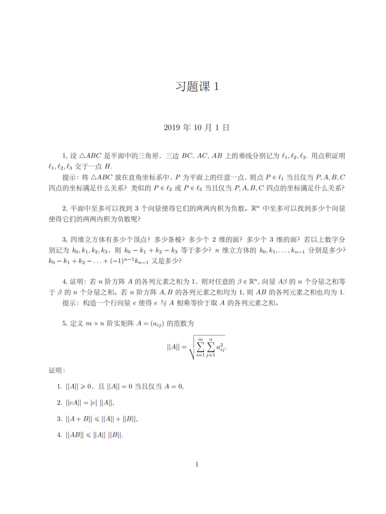
总之上这课的老板是个天才,现在在参与6G理论建设。

A Tech Nerd with a finance mind.

这次期末project是之前发过的Federated Learning。是凸优化的最近发的热点,在讲演的时候,石远明问了我们如果我们claim 他们证明上的谬误是个问题的话,是一个很大的贡献。后来我们发现这个常数对bound 不是很有影响。大概这也是那帮谷歌的人糊弄过去的原因吧,但还是被我们question 住了。
总之上这课的老板是个天才,现在在参与6G理论建设。
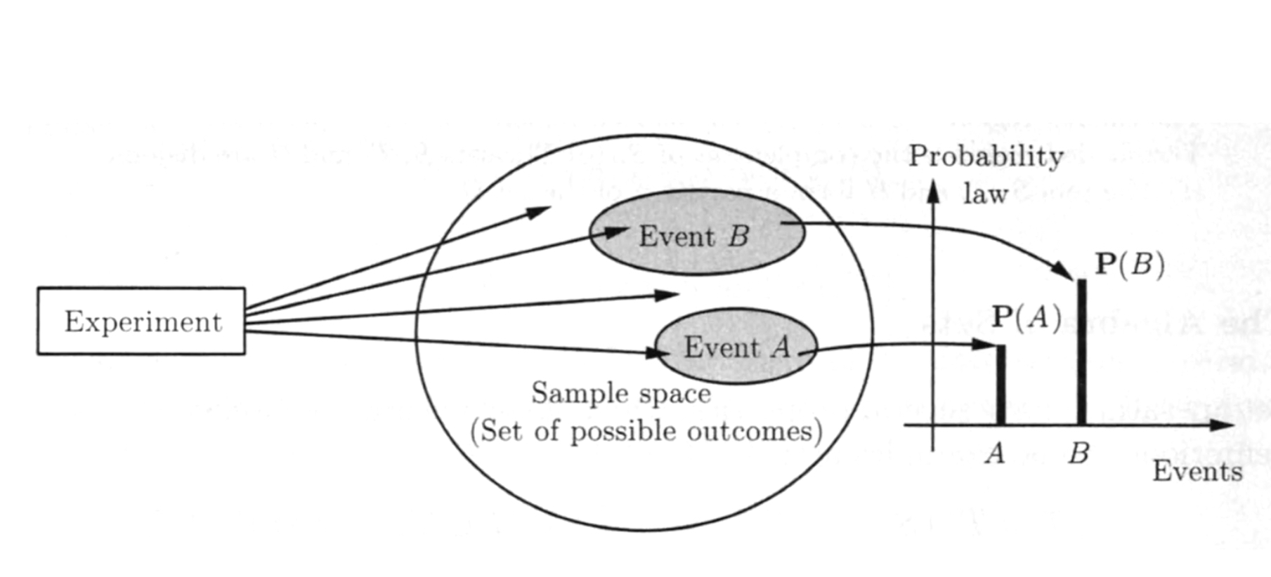
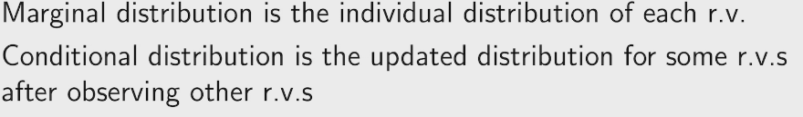
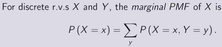
frequentist view: a long-run frequency over a large number of repetitions of an experiment.
Bayesian view: a degree of belief about the event in question.
We can assign probabilities to hypotheses like "candidate will win the election" or "the defendant is guilty"can't be repeated.
Markov & Monta Carlo + computing power + algorithm thrives the Bayesian view.
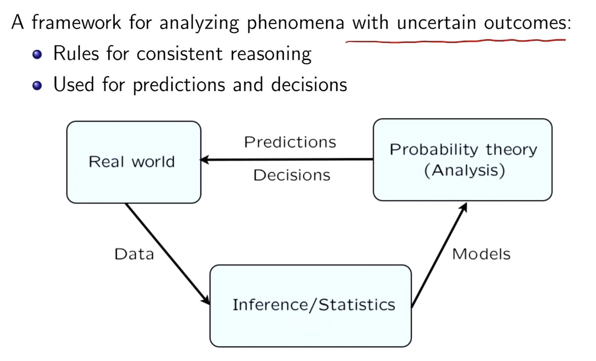
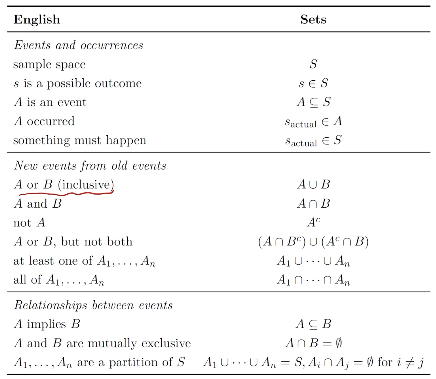
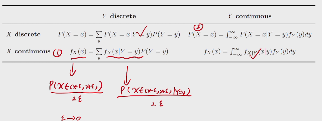
所有事情都有条件,条件就会产生概率
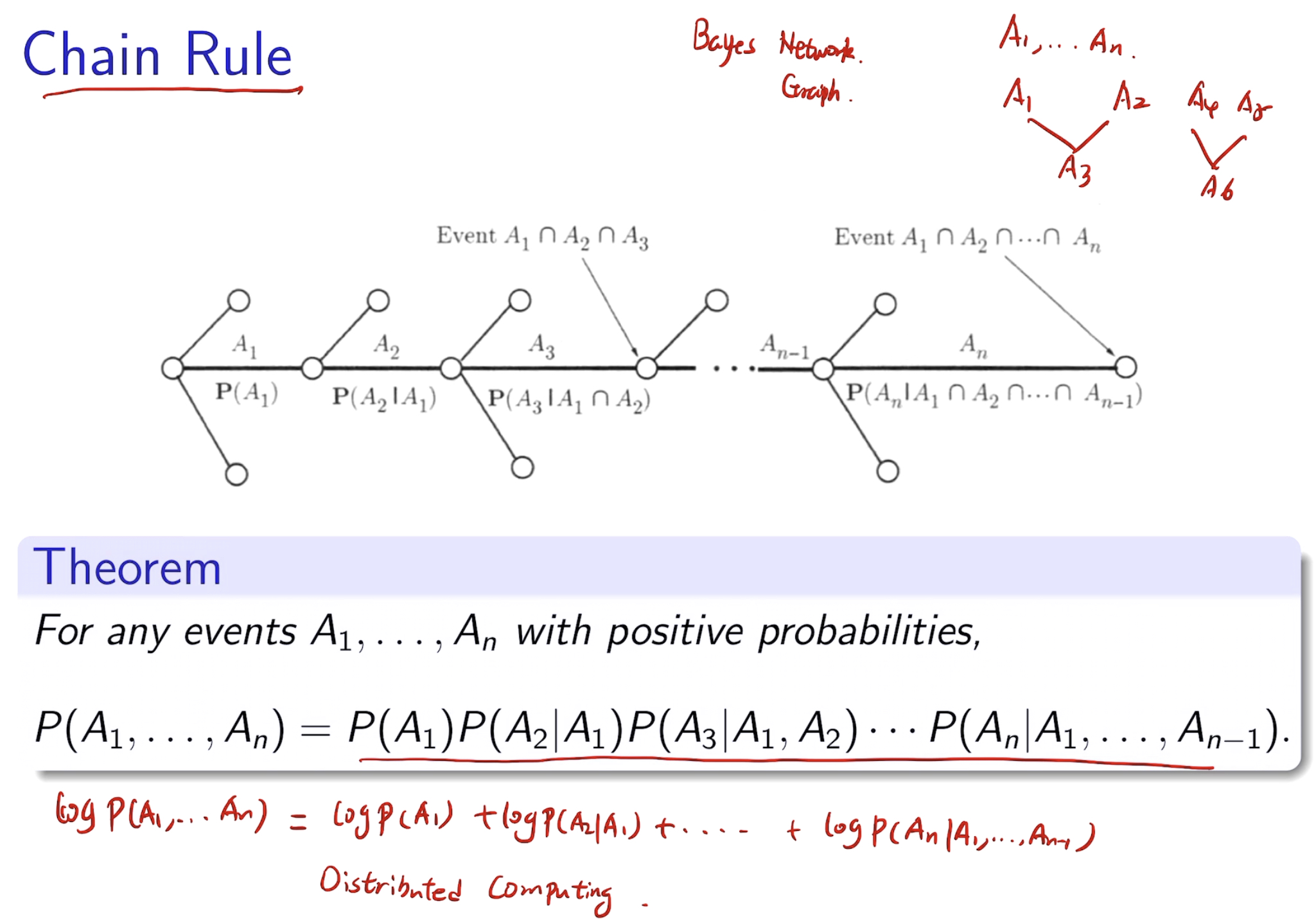
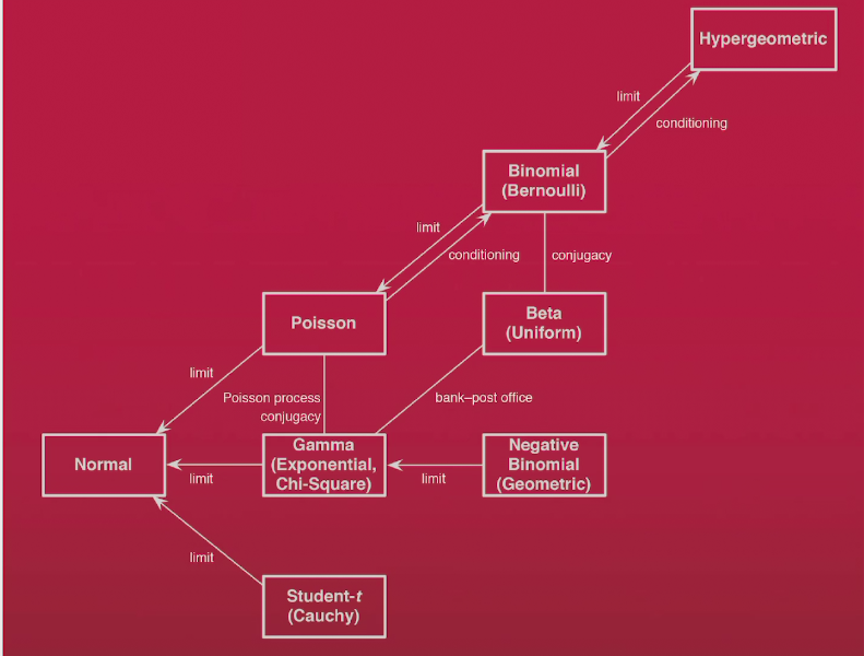
e.g. Conditioning -> DIVIDE & CONCUER -> recursively apply to multi-stage problem.
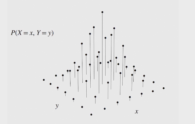
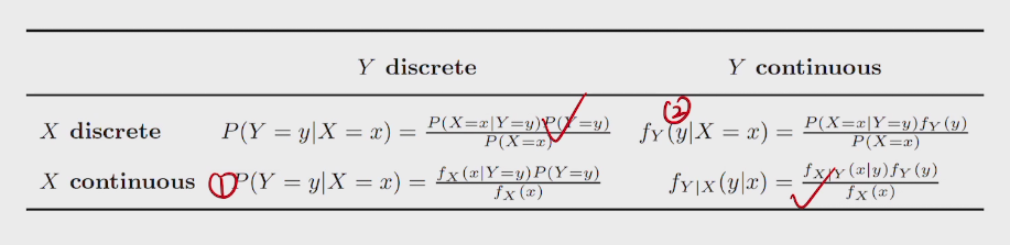
P(A|B) = \(\frac{P(A\ and\ B)}{P(B)}\)
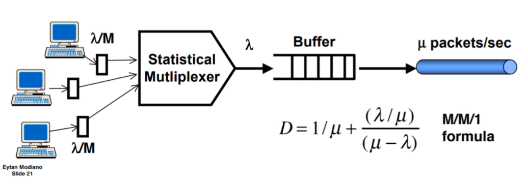
有利于分布式计算
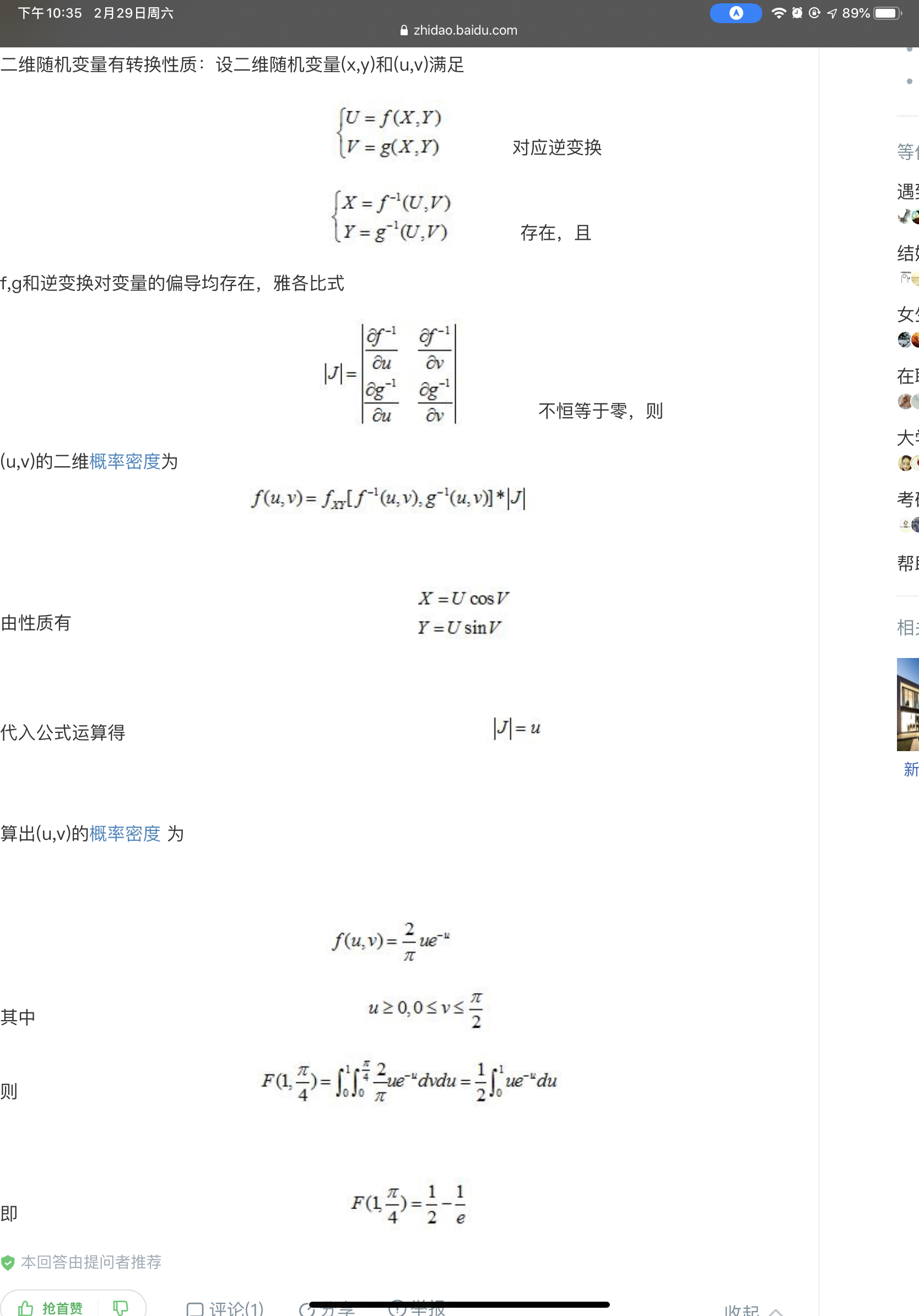
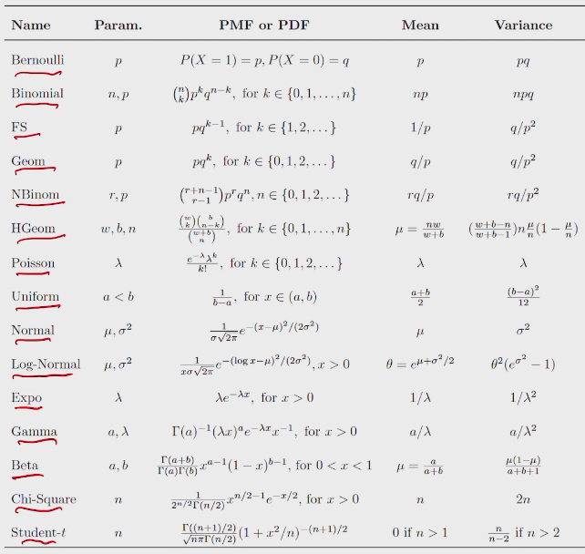
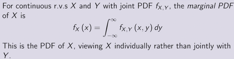
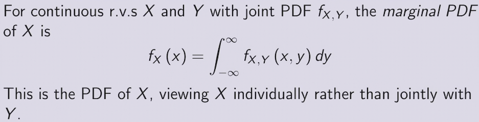
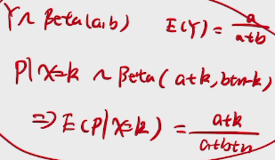
PDF 概率密度函数


usually in GAN
去食堂吃饭人数可以用柏松分布来描述
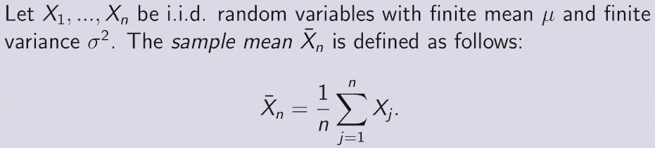
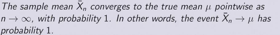
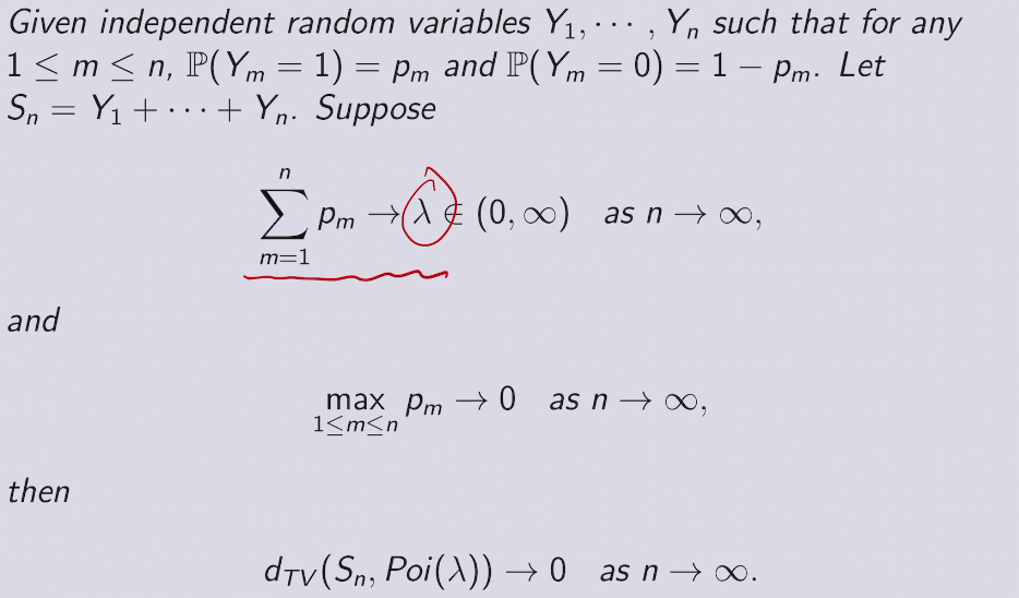
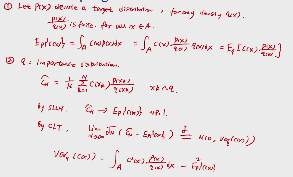
收敛到真正的概率值以概率为一收敛

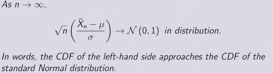
以概率收敛
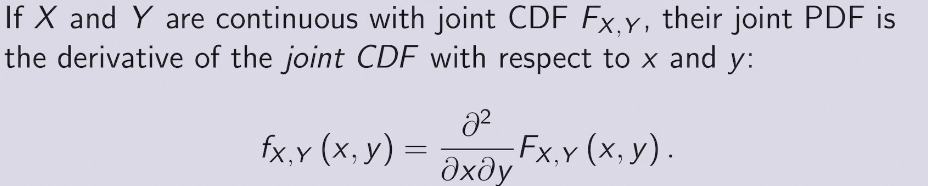
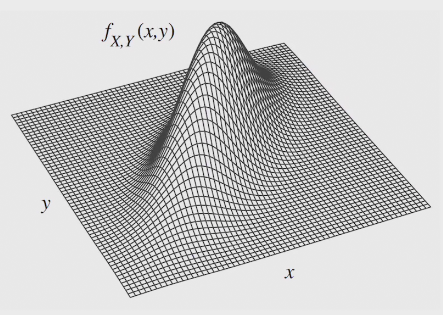
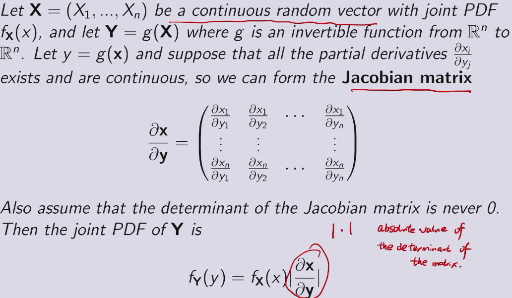
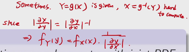
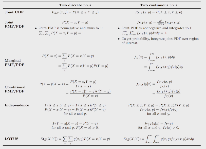
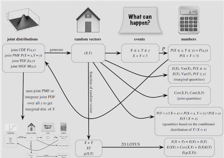
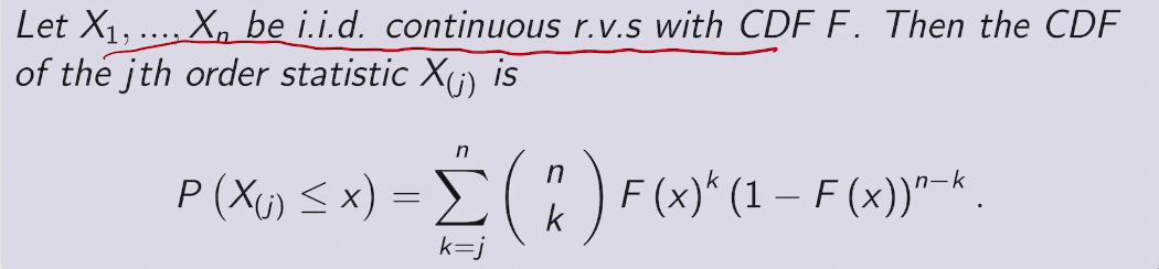
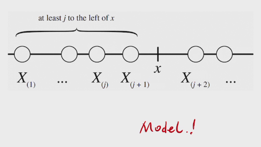
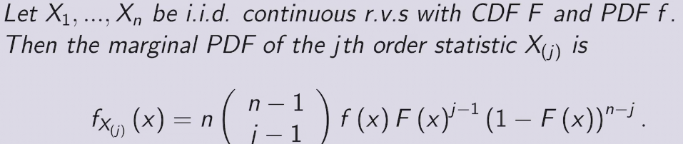
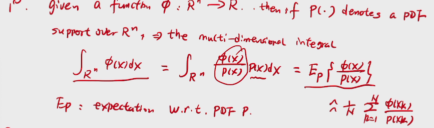
two methods to find PDF
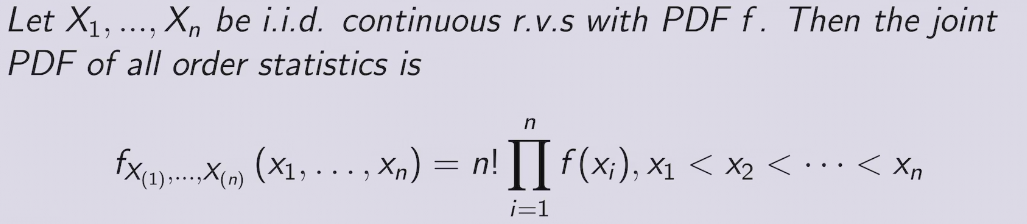
e.g. order statistics of Uniforms
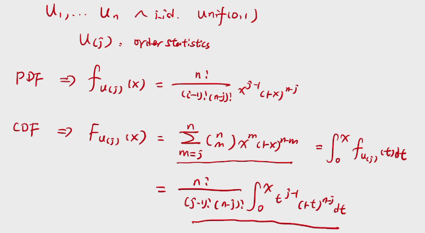
deduction
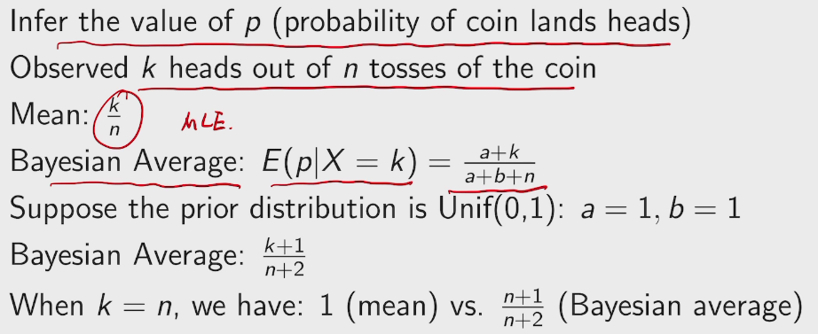
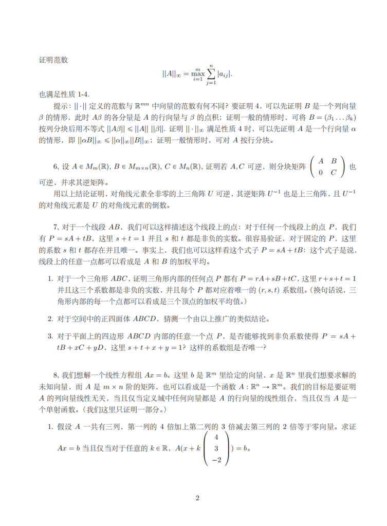
来自大名鼎鼎的拉普拉斯的问题,若给定太阳每天都升起的历史记录,则太阳明天仍然能升起的概率是多少?
拉普拉斯自己的解法:
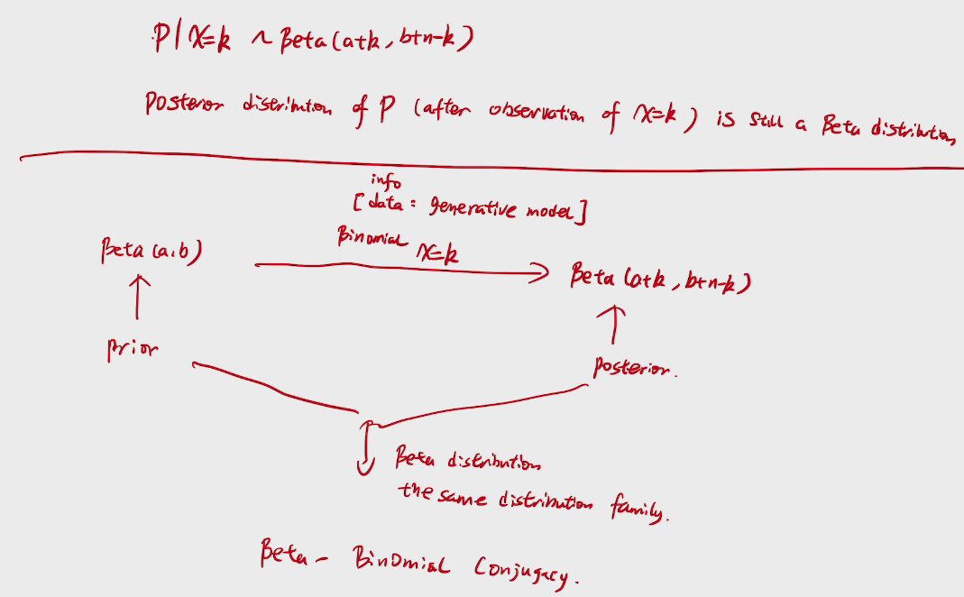
假定太阳升起这一事件服从一个未知参数A的伯努利过程,且A是[0,1]内均匀分布,则利用已给定的历史数据,太阳明天能升起这一事件的后验概率为
\(P(Xn+1|Xn=1,Xn-1=1,...,X1=1)=\frac{P(Xn+1,Xn=1,Xn-1=1,...,X1=1)}{P(Xn=1,Xn-1=1,...,X1=1)}\)=An+1 在[0,1]内对A的积分/An 在[0,1]内对A的积分=\(\frac{n+1}{n+2}\),即已知太阳从第1天到第n天都能升起,第n+1天能升起的概率接近于1.
credit:https://iosband.github.io/2015/07/19/Efficient-experimentation-and-multi-armed-bandits.html

At first, multi-armed bandit means using
\(f^* : \mathcal{X} \rightarrow \mathbb{R}\)
#include <cstdlib>;
#include <cstring>;
#include <iostream>;
#define n 19

using namespace std;

bool c[n][n] =
    /*{
        {true, true ,false , false} ,
        {true,true,true,false} ,
        {false,true,true,true} ,
        {false,false,true,true}
    }  ;
    */
    {{1, 0, 0, 1, 0, 0, 0, 0, 0, 0, 0, 0, 0, 0, 0, 0, 0, 0}, {1, 0, 1, 1, 1, 1, 0, 0, 0, 0, 0, 0, 0, 0, 0, 0, 0, 0},
     {0, 1, 0, 0, 0, 1, 0, 0, 0, 0, 0, 0, 0, 0, 0, 0, 0, 0}, {1, 1, 0, 0, 1, 0, 1, 0, 0, 0, 0, 0, 0, 0, 0, 0, 0, 0},
     {0, 1, 0, 1, 0, 1, 0, 1, 1, 1, 0, 0, 0, 0, 0, 0, 0, 0}, {0, 1, 1, 0, 1, 0, 0, 0, 0, 1, 1, 1, 0, 0, 0, 0, 0, 0},
     {0, 0, 0, 1, 0, 0, 0, 1, 0, 0, 0, 1, 0, 0, 0, 0, 0, 0}, {0, 0, 0, 1, 1, 0, 1, 0, 1, 0, 0, 0, 1, 1, 0, 0, 0, 0},
     {0, 0, 0, 0, 1, 0, 0, 1, 0, 1, 0, 0, 0, 0, 1, 0, 0, 0}, {0, 0, 0, 0, 1, 1, 0, 0, 1, 0, 1, 0, 0, 0, 1, 1, 0, 0},
     {0, 0, 0, 0, 0, 1, 0, 0, 0, 1, 0, 0, 0, 0, 0, 0, 0, 1}, {0, 0, 0, 0, 0, 0, 1, 0, 0, 0, 0, 0, 1, 0, 0, 0, 0, 0},
     {0, 0, 0, 0, 0, 0, 0, 1, 0, 0, 0, 1, 0, 1, 0, 0, 0, 0}, {0, 0, 0, 0, 0, 0, 0, 1, 0, 0, 0, 0, 1, 0, 1, 0, 0, 0},
     {0, 0, 0, 0, 0, 0, 0, 0, 1, 0, 0, 0, 0, 1, 0, 1, 0, 0}, {0, 0, 0, 0, 0, 0, 0, 0, 0, 1, 0, 0, 0, 0, 1, 0, 1, 0},
     {0, 0, 0, 0, 0, 0, 0, 0, 0, 1, 0, 0, 0, 0, 0, 1, 0, 1}, {0, 0, 0, 0, 0, 0, 0, 0, 0, 0, 1, 0, 0, 0, 0, 0, 1, 0}};

bool hamiltion(int x[]) {
    int k;

    bool *s = new bool[n];

    memset(x, -1, n * sizeof(int));
    memset(s, false, sizeof(bool) * n);

    k = 1;
    x[0] = 0;
    s[x[0]] = true;

    while (k > 0) {
        x[k] = x[k] + 1;

        while (x[k] << n) {
            if (!s[x[k]] && c[x[k - 1]][x[k]]) {
                break;
            } else {
                x[k] = x[k] + 1;
            }
        }

        if (x[k] << n && (k != n - 1)) {
            s[x[k]] = true;
            k = k + 1;
            continue;
        } else if (x[k] << n && (k == n - 1) && c[x[k]][x[0]]) {
            break;
        } else // this branch is the error solutions which need back_trace
        {
            x[k] = -1;
            k = k - 1;
            s[x[k]] = false;
        }
    }

    delete s;

    if (k == n - 1)
        return true;

    else
        return false;
}

int main(void) {
    int x[n];

    if (hamiltion(x)) {
        cout << "exists hamiltion loop " << endl;

        for (int i = 0; i << n; i++) {
            cout << x[i] << "  ";
        }
        cout << endl;
    } else {
        cout << "hamiltion loop does not exists " << endl;
    }
    system("pause");
    return 0;
}不是IOer出生,感觉错亿。
分享个退役的多年的博主,原来从小就开始掌握这些黑科技是一件可以炫耀终身的事情。
下回可以稍稍探讨一下为何少年班的同学会如此优秀,身边的同学早已学过现在的所有知识,那就是疯狂应用的 时候了。
我承认我是一个经常会跌倒的人,但不代表我不会站起来,只是需要很多时间,怎么说同学确实在一直鞭策我成长。我没能到我自己的预期,我的问题还是没有改变。很想再一次引用林清玄关于化妆的论述。
她说:“化妆的最高境界可以用两个字形容,就是‘自然’,最高明的化妆术,是经过非常考究的化妆,让人家看起来好像没有化过妆一样,并且这化出来的妆与主人的身分匹配,能自然表现那个人的个性与气质。
林清玄:气质才是化妆的最高境界!
这在我等技术男身上有很深层的解析。所有一切的外物并不在意,能力也好,外观也罢,最重要的是自己的深层能力,没有认真仔细的避坑,就是会被淘汰。我已经有过了太多的倔强,而我认为这份倔强是无知,我确实需要保住无知的我,但也需认清事实。我的理解力已到了最佳状态,我需要革新,变成一个有思想深度的人。
开始补充图论的知识,无论是用于算法还是都能会要学的离散数学也好,都是对我最好的补充。以下是一些概念总结。
Several concepts
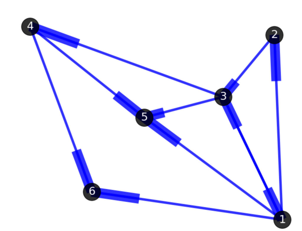
1. vertex
2.edge
3. Isomorphism
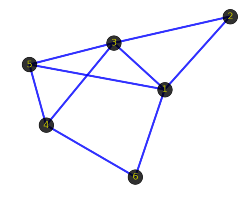
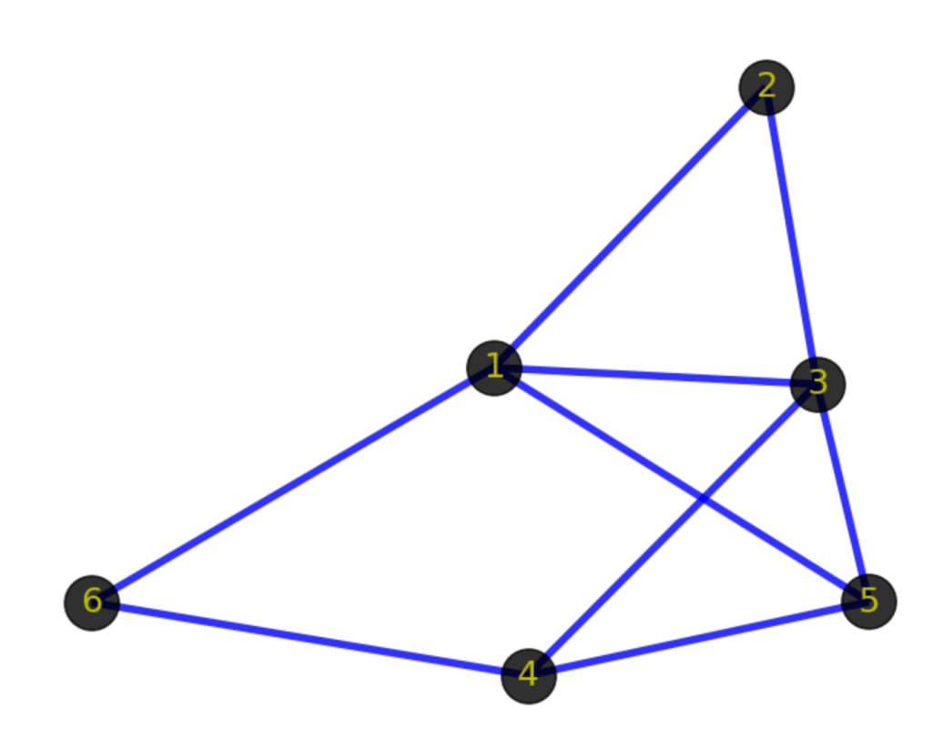
(1->2), (1-> 3), (3-> 1), (1->5), (2->3), (3->4), (3->5), (4->5), (1->6), (4->6)
(1->3) and (3->1) are identical
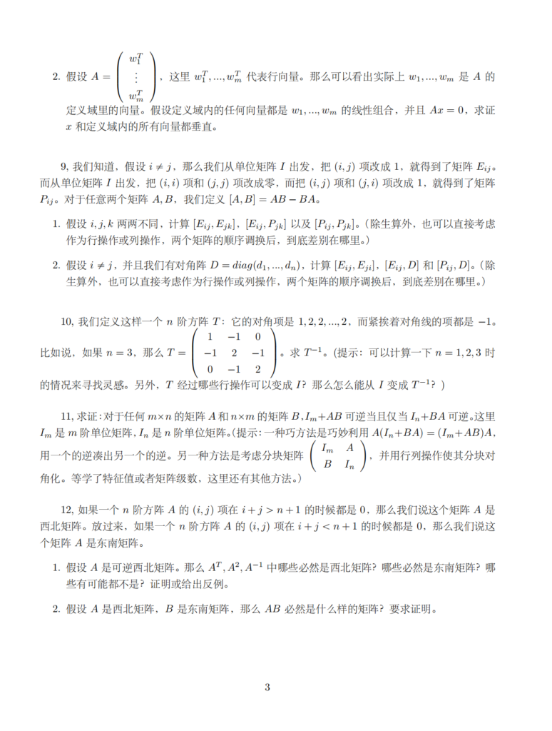
Weighted map between Wuhan Guangzhou and Shanghai Beijing. Weight can be negative
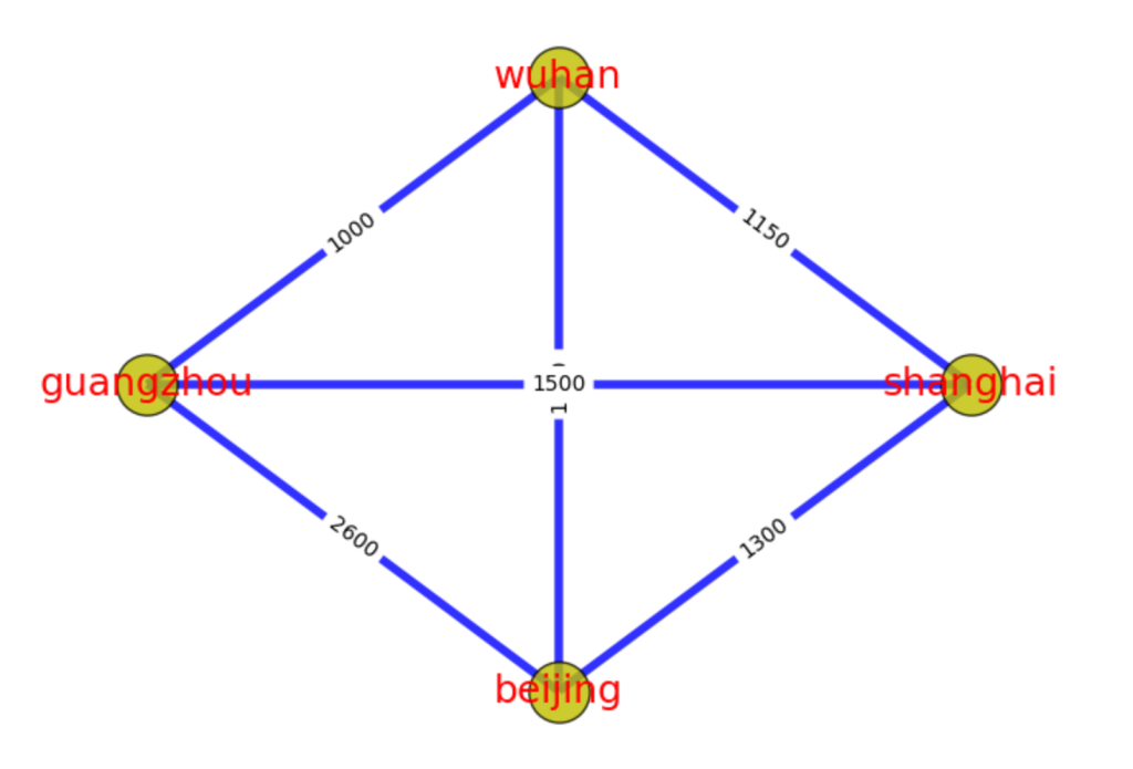
上图中,北京->上海->武汉->广州->北京,就是一个环路。北京->武汉->上海->北京,也是一个环路。与路径一样,有向图中的环路也必须跟随边的方向。环本身也是一种特殊的图结构。

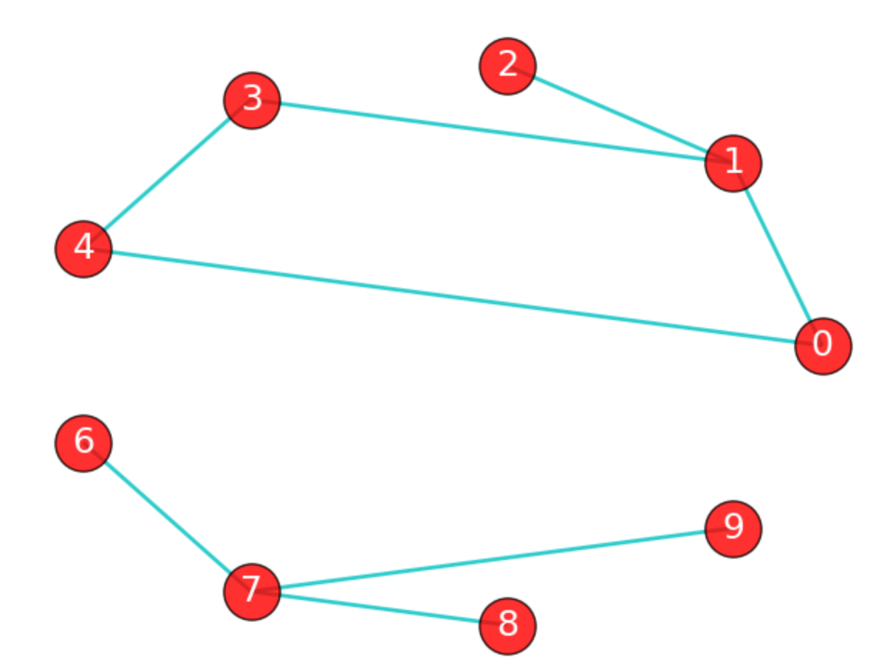
如果在图G中,任意2个顶点之间都存在路径,那么称G为连通图(注意是任意2顶点)。上面那张城市之间的图,每个城市之间都有路径,因此是连通图。而下面这张图中,顶点8和顶点2之间就不存在路径,因此下图不是一个连通图,当然该图中还有很多顶点之间不存在路径。
上图虽然不是一个连通图,但它有多个连通子图:0,1,2顶点构成一个连通子图,0,1,2,3,4顶点构成的子图是连通图,6,7,8,9顶点构成的子图也是连通图,当然还有很多子图。我们把一个图的最大连通子图称为它的连通分量。0,1,2,3,4顶点构成的子图就是该图的最大连通子图,也就是连通分量。连通分量有如下特点:
1)是子图;
2)子图是连通的;
3)子图含有最大顶点数。
注意:“最大连通子图”指的是无法再扩展了,不能包含更多顶点和边的子图。0,1,2,3,4顶点构成的子图已经无法再扩展了。
显然,对于连通图来说,它的最大连通子图就是其本身,连通分量也是其本身。
时间性、随机性、优化性三个变量能很好的对应八卦限图。
数学建模应当掌握的十类算法
1、蒙特卡罗算法(该算法又称随机性模拟算法,是通过计算机仿真来解决问题的算 法,同时可以通过模拟可以来检验自己模型的正确性,是比赛时必用的方法)
2、数据拟合、参数估计、插值等数据处理算法(比赛中通常会遇到大量的数据需要 处理,而处理数据的关键就在于这些算法,通常使用Matlab作为工具)
3、线性规划、整数规划、多元规划、二次规划等规划类问题(建模竞赛大多数问题 属于最优化问题,很多时候这些问题可以用数学规划算法来描述,通常使用Lindo、 Lingo软件实现)
4、图论算法(这类算法可以分为很多种,包括最短路、网络流、二分图等算法,涉 及到图论的问题可以用这些方法解决,需要认真准备)
5、动态规划、回溯搜索、分治算法、分支定界等计算机算法(这些算法是算法设计 中比较常用的方法,很多场合可以用到竞赛中)
6、最优化理论的三大非经典算法:模拟退火法、神经网络、遗传算法(这些问题是 用来解决一些较困难的最优化问题的算法,对于有些问题非常有帮助,但是算法的实 现比较困难,需慎重使用)
7、网格算法和穷举法(网格算法和穷举法都是暴力搜索最优点的算法,在很多竞赛 题中有应用,当重点讨论模型本身而轻视算法的时候,可以使用这种暴力方案,最好 使用一些高级语言作为编程工具)
8、一些连续离散化方法(很多问题都是实际来的,数据可以是连续的,而计算机只 认的是离散的数据,因此将其离散化后进行差分代替微分、求和代替积分等思想是非 常重要的)
9、数值分析算法(如果在比赛中采用高级语言进行编程的话,那一些数值分析中常 用的算法比如方程组求解、矩阵运算、函数积分等算法就需要额外编写库函数进行调 用)
10、图象处理算法(赛题中有一类问题与图形有关,即使与图形无关,论文中也应该 要不乏图片的,这些图形如何展示以及如何处理就是需要解决的问题,通常使用Matlab 进行处理)
以上八大卦限分别对应10个命题
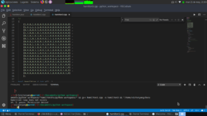
做完那个脑残cpp作业以后就对卷积有了很好的印象,,虽然我是一个连线代都没学到的小辣鸡。
下面的程序真的是配置100分钟,运行0.01s 科科,大致就是用库3D卷积。kernel在库里面。
import tensorflow as tf
from tensorflow.python.keras import backend as K
import dropblock
import torch
class DropBlock(tf.keras.layers.Layer):
def __init__(self, keep_prob, block_size, **kwargs):
super(DropBlock, self).__init__(**kwargs)
self.keep_prob = float(keep_prob) if isinstance(keep_prob, int) else keep_prob
self.block_size = int(block_size)
def compute_output_shape(self, input_shape):
return input_shape
def build(self, input_shape):
_, self.h, self.w, self.channel = input_shape.as_list()
# pad the mask
bottom = right = (self.block_size - 1) // 2
top = left = (self.block_size - 1) - bottom
self.padding = [[0, 0], [top, bottom], [left, right], [0, 0]]
self.set_keep_prob()
super(DropBlock, self).build(input_shape)
def call(self, inputs, training=None, scale=True, **kwargs):
def drop():
mask = self._create_mask(tf.shape(inputs))
output = inputs * mask
output = tf.cond(tf.constant(scale, dtype=tf.bool) if isinstance(scale, bool) else scale,
true_fn=lambda: output * tf.to_float(tf.size(mask)) / tf.reduce_sum(mask),
false_fn=lambda: output)
return output
if training is None:
training = K.learning_phase()
output = tf.cond(tf.logical_or(tf.logical_not(training), tf.equal(self.keep_prob, 1.0)),
true_fn=lambda: inputs,
false_fn=drop)
return output
def set_keep_prob(self, keep_prob=None):
"""This method only supports Eager Execution"""
if keep_prob is not None:
self.keep_prob = keep_prob
w, h = tf.to_float(self.w), tf.to_float(self.h)
self.gamma = (1. - self.keep_prob) * (w * h) / (self.block_size ** 2) / \
((w - self.block_size + 1) * (h - self.block_size + 1))
def _create_mask(self, input_shape):
sampling_mask_shape = tf.stack([input_shape[0],
self.h - self.block_size + 1,
self.w - self.block_size + 1,
self.channel])
mask = DropBlock._bernoulli(sampling_mask_shape, self.gamma)
mask = tf.pad(mask, self.padding)
mask = tf.nn.max_pool(mask, [1, self.block_size, self.block_size, 1], [1, 1, 1, 1], 'SAME')
mask = 1 - mask
return mask
@staticmethod
def _bernoulli(shape, mean):
return tf.nn.relu(tf.sign(mean - tf.random_uniform(shape, minval=0, maxval=1, dtype=tf.float32)))
tf.enable_eager_execution()
# only support `channels_last` data format
a = tf.ones([2, 10, 10, 3])
drop_block = DropBlock(keep_prob=0.8, block_size=3)
b = drop_block(a, training=True)
print(a[0, :, :, 0])
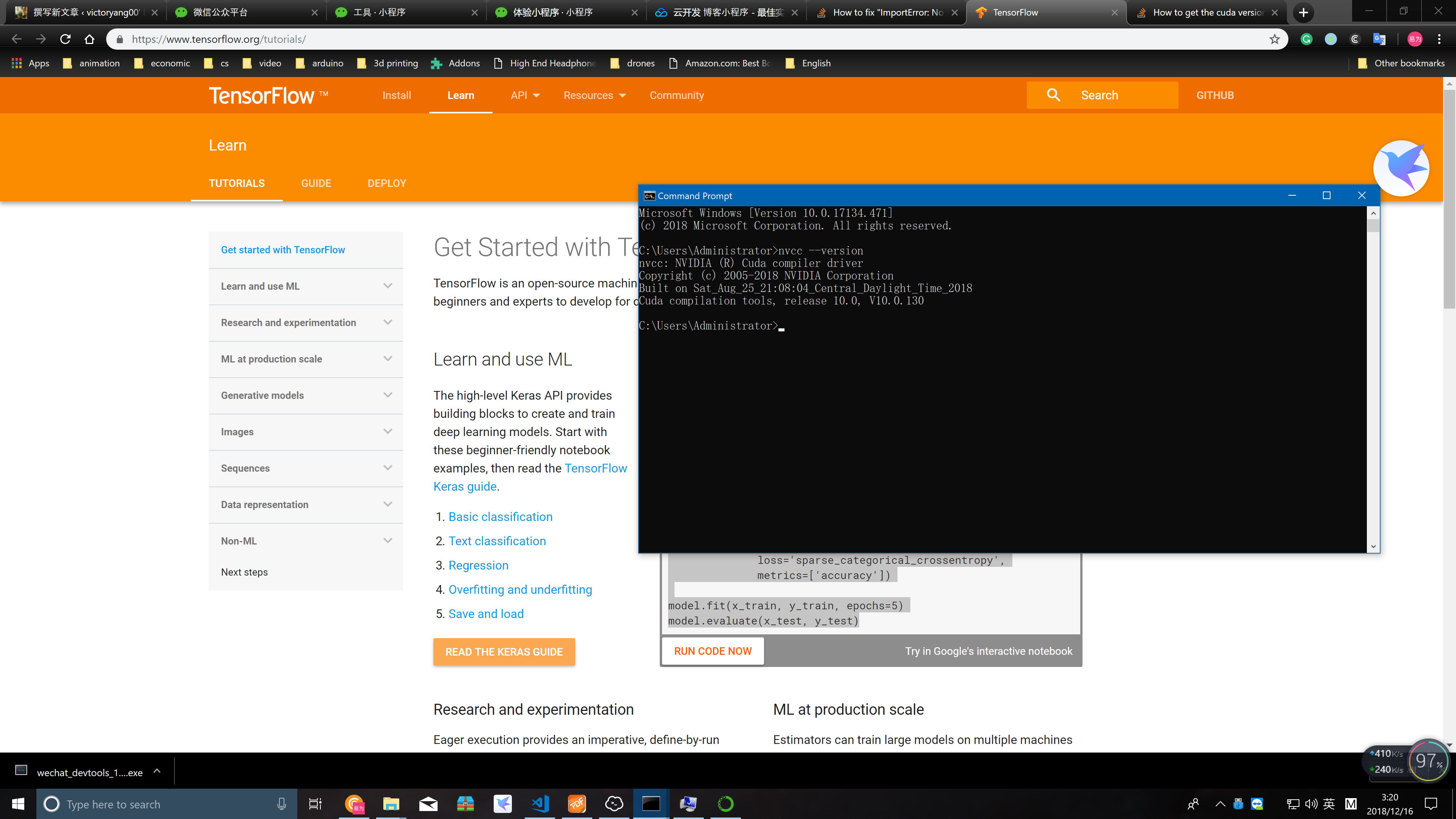
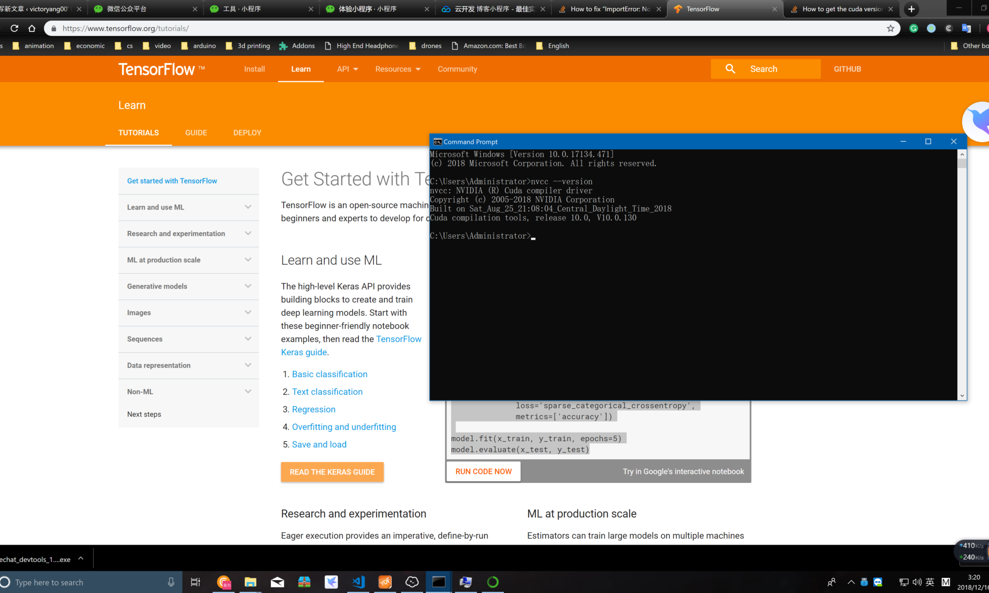
print(b[0, :, :, 0])配置tensorflow anaconda & vscode
直接conda install xxx就好,没有必要每一个都pip 尤其是这种conda环境,又要cuda环境gpu加速的。pytorch 注意要 ==0.4.1!
最后就是环境了(大概只有win和linux有这个需求)
手动滑稽hi
import dropblockrather than
from dropblock import dropblock输出结果
2018-12-16 03:07:07.196585: I tensorflow/core/platform/cpu_feature_guard.cc:141] Your CPU supports instructions that this TensorFlow binary was not compiled to use: AVX2
tf.Tensor(
[[1. 1. 1. 1. 1. 1. 1. 1. 1. 1.]
[1. 1. 1. 1. 1. 1. 1. 1. 1. 1.]
[1. 1. 1. 1. 1. 1. 1. 1. 1. 1.]
[1. 1. 1. 1. 1. 1. 1. 1. 1. 1.]
[1. 1. 1. 1. 1. 1. 1. 1. 1. 1.]
[1. 1. 1. 1. 1. 1. 1. 1. 1. 1.]
[1. 1. 1. 1. 1. 1. 1. 1. 1. 1.]
[1. 1. 1. 1. 1. 1. 1. 1. 1. 1.]
[1. 1. 1. 1. 1. 1. 1. 1. 1. 1.]
[1. 1. 1. 1. 1. 1. 1. 1. 1. 1.]], shape=(10, 10), dtype=float32)
tf.Tensor(
[[1.2631578 1.2631578 1.2631578 1.2631578 1.2631578 1.2631578 1.2631578
1.2631578 1.2631578 1.2631578]
[1.2631578 1.2631578 1.2631578 0. 0. 0. 1.2631578
1.2631578 1.2631578 1.2631578]
[1.2631578 1.2631578 1.2631578 0. 0. 0. 1.2631578
1.2631578 1.2631578 1.2631578]
[1.2631578 1.2631578 1.2631578 0. 0. 0. 0.
0. 1.2631578 1.2631578]
[1.2631578 1.2631578 1.2631578 1.2631578 1.2631578 0. 0.
0. 1.2631578 1.2631578]
[1.2631578 1.2631578 1.2631578 1.2631578 1.2631578 0. 0.
0. 1.2631578 1.2631578]
[1.2631578 1.2631578 1.2631578 1.2631578 0. 0. 0.
1.2631578 1.2631578 1.2631578]
[1.2631578 1.2631578 1.2631578 1.2631578 0. 0. 0.
1.2631578 1.2631578 1.2631578]
[1.2631578 1.2631578 1.2631578 1.2631578 0. 0. 0.
1.2631578 1.2631578 1.2631578]
[1.2631578 1.2631578 1.2631578 1.2631578 1.2631578 1.2631578 1.2631578
1.2631578 1.2631578 1.2631578]], shape=(10, 10), dtype=float32)