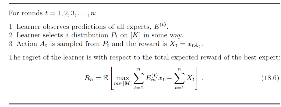
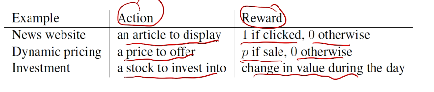
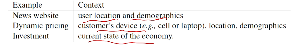
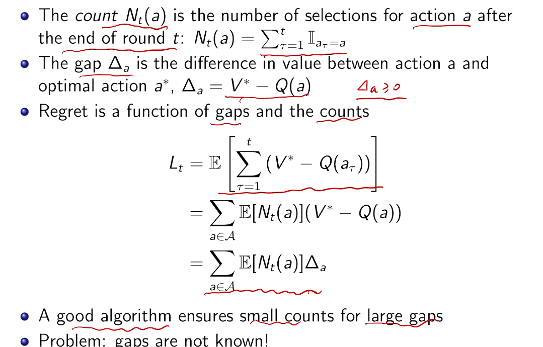
a novel way to read from tar volume

intro

some of the volume is right in the root folder of the tar, for example.

.
├── AUTHORS
├── boards
│   ├── arm64.gni
│   ├── as370.gni
│   ├── BUILD.gn
│   ├── c18.gni
│   ├── chromebook-x64.gni
│   ├── cleo.gni
│   ├── hikey960.gni
│   ├── kirin970.gni
│   ├── msm8998.gni
│   ├── msm8x53-som.gni
│   ├── mt8167s_ref.gni
│   ├── OWNERS
│   ├── qemu-arm64.gni
│   ├── qemu-x64.gni
│   ├── toulouse.gni
│   ├── vim2.gni
│   ├── vim3.gni
│   ├── vs680.gni
│   └── x64.gni
├── build
│   ├── banjo
│   │   ├── banjo.gni
│   │   ├── banjo_library.gni
│   │   ├── BUILD.gn
│   │   ├── gen_response_file.py
│   │   ├── gen_sdk_meta.py
│   │   └── toolchain.gni
│   ├── bind
│   │   └── bind.gni
│   ├── board.gni
│   ├── BUILD.gn
│   ├── build_id.gni
│   ├── c
│   │   ├── banjo_c.gni
│   │   ├── BUILD.gn
│   │   └── fidl_c.gni
│   ├── cat.sh
│   ├── cipd.gni
│   ├── cmake
│   │   ├── HostLinuxToolchain.cmake
│   │   ├── README.md
│   │   └── ToolchainCommon.cmake
│   ├── cmx
│   │   ├── block_deprecated_misc_storage.json
│   │   ├── block_deprecated_shell.json
│   │   ├── block_rootjob_svc.json
│   │   ├── block_rootresource_svc.json
│   │   ├── cmx.gni
│   │   ├── facets
│   │   │   └── module_facet_schema.json
│   │   ├── internal_allow_global_data.cmx
│   │   └── OWNERS
│   ├── compiled_action.gni
│   ├── config
│   │   ├── arm.gni
│   │   ├── BUILDCONFIG.gn
│   │   ├── BUILD.gn
│   │   ├── clang
│   │   │   └── clang.gni
│   │   ├── compiler.gni
│   │   ├── fuchsia
│   │   │   ├── BUILD.gn
│   │   │   ├── rules.gni
│   │   │   ├── sdk.gni
│   │   │   ├── zbi.gni
│   │   │   ├── zircon.gni
│   │   │   ├── zircon_images.gni
│   │   │   └── zircon_legacy_vars.gni
│   │   ├── host_byteorder.gni
│   │   ├── linux
│   │   │   └── BUILD.gn
│   │   ├── lto
│   │   │   ├── BUILD.gn
│   │   │   └── config.gni
│   │   ├── mac
│   │   │   ├── BUILD.gn
│   │   │   ├── mac_sdk.gni
│   │   │   └── package_framework.py
│   │   ├── OWNERS
│   │   ├── profile
│   │   │   └── BUILD.gn
│   │   ├── sanitizers
│   │   │   ├── asan_default_options.c
│   │   │   ├── BUILD.gn
│   │   │   ├── debugdata.cmx
│   │   │   └── ubsan_default_options.c
│   │   ├── scudo
│   │   │   ├── BUILD.gn
│   │   │   ├── scudo_default_options.c
│   │   │   └── scudo.gni
│   │   └── sysroot.gni
│   ├── config.gni
│   ├── cpp
│   │   ├── binaries.py
│   │   ├── BUILD.gn
│   │   ├── extract_imported_symbols.gni
│   │   ├── extract_imported_symbols.sh
│   │   ├── extract_public_symbols.gni
│   │   ├── extract_public_symbols.sh
│   │   ├── fidl_cpp.gni
│   │   ├── fidlmerge_cpp.gni
│   │   ├── gen_sdk_prebuilt_meta_file.py
│   │   ├── gen_sdk_sources_meta_file.py
│   │   ├── sdk_executable.gni
│   │   ├── sdk_shared_library.gni
│   │   ├── sdk_source_set.gni
│   │   ├── sdk_static_library.gni
│   │   ├── verify_imported_symbols.gni
│   │   ├── verify_imported_symbols.sh
│   │   ├── verify_pragma_once.gni
│   │   ├── verify_pragma_once.py
│   │   ├── verify_public_symbols.gni
│   │   ├── verify_public_symbols.sh
│   │   └── verify_runtime_deps.py
│   ├── dart
│   │   ├── BUILD.gn
│   │   ├── dart.gni
│   │   ├── dart_library.gni
│   │   ├── dart_remote_test.gni
│   │   ├── dart_tool.gni
│   │   ├── empty_pubspec.yaml
│   │   ├── fidl_dart.gni
│   │   ├── fidlmerge_dart.gni
│   │   ├── gen_analyzer_invocation.py
│   │   ├── gen_app_invocation.py
│   │   ├── gen_dart_test_invocation.py
│   │   ├── gen_dot_packages.py
│   │   ├── gen_remote_test_invocation.py
│   │   ├── gen_test_invocation.py
│   │   ├── group_tests.py
│   │   ├── label_to_package_name.py
│   │   ├── OWNERS
│   │   ├── run_analysis.py
│   │   ├── sdk
│   │   │   ├── detect_api_changes
│   │   │   │   ├── analysis_options.yaml
│   │   │   │   ├── bin
│   │   │   │   │   └── main.dart
│   │   │   │   ├── BUILD.gn
│   │   │   │   ├── lib
│   │   │   │   │   ├── analyze.dart
│   │   │   │   │   ├── diff.dart
│   │   │   │   │   └── src
│   │   │   │   │       └── visitor.dart
│   │   │   │   ├── pubspec.yaml
│   │   │   │   ├── schema.json
│   │   │   │   └── test
│   │   │   │       ├── analyze_test.dart
│   │   │   │       └── diff_test.dart
│   │   │   ├── gen_meta_file.py
│   │   │   └── sort_deps.py
│   │   ├── test.gni
│   │   ├── toolchain.gni
│   │   └── verify_sources.py
│   ├── development.key
│   ├── driver_package.gni
│   ├── fidl
│   │   ├── BUILD.gn
│   │   ├── fidl.gni
│   │   ├── fidl_library.gni
│   │   ├── gen_response_file.py
│   │   ├── gen_sdk_meta.py
│   │   ├── linting_exceptions.gni
│   │   ├── OWNERS
│   │   ├── run_and_gen_stamp.sh
│   │   ├── toolchain.gni
│   │   └── wireformat.gni
│   ├── fuchsia
│   │   └── sdk.gni
│   ├── Fuchsia.cmake
│   ├── fuzzing
│   │   ├── BUILD.gn
│   │   ├── fuzzer.gni
│   │   └── OWNERS
│   ├── gn
│   │   ├── BUILD.gn
│   │   ├── gen_persistent_log_config.py
│   │   ├── OWNERS
│   │   ├── unpack_build_id_archives.sh
│   │   └── write_package_json.py
│   ├── gn_helpers.py
│   ├── gn_run_binary.sh
│   ├── go
│   │   ├── BUILD.gn
│   │   ├── build.py
│   │   ├── fidl_go.gni
│   │   ├── gen_library_metadata.py
│   │   ├── go_binary.gni
│   │   ├── go_build.gni
│   │   ├── go_fuzzer.gni
│   │   ├── go_fuzzer_wrapper.go
│   │   ├── go_library.gni
│   │   ├── go_test.gni
│   │   ├── OWNERS
│   │   └── toolchain.gni
│   ├── gypi_to_gn.py
│   ├── host.gni
│   ├── images
│   │   ├── add_tag_to_manifest.sh
│   │   ├── args.gni
│   │   ├── assemble_system.gni
│   │   ├── boot.gni
│   │   ├── bringup
│   │   │   └── BUILD.gn
│   │   ├── BUILD.gn
│   │   ├── collect_blob_manifest.gni
│   │   ├── create-shell-commands.py
│   │   ├── custom_signing.gni
│   │   ├── dummy
│   │   │   └── example.txt
│   │   ├── efi_local_cmdline.txt
│   │   ├── elfinfo.py
│   │   ├── filesystem_limits.gni
│   │   ├── finalize_manifests.py
│   │   ├── format_filesystem_sizes.py
│   │   ├── fvm.gni
│   │   ├── generate_flash_script.sh
│   │   ├── guest
│   │   │   ├── BUILD.gn
│   │   │   └── guest_meta_package.json
│   │   ├── manifest_add_dest_prefix.sh
│   │   ├── manifest_content_expand.sh
│   │   ├── manifest.gni
│   │   ├── manifest_list_collect_unique_blobs.py
│   │   ├── manifest.py
│   │   ├── max_fvm_size.gni
│   │   ├── OWNERS
│   │   ├── pack-images.py
│   │   ├── pkgfs.gni
│   │   ├── recovery
│   │   │   └── BUILD.gn
│   │   ├── shell_commands.gni
│   │   ├── system_image_prime_meta_package.json
│   │   ├── system_meta_package.json
│   │   ├── ta.gni
│   │   ├── update_package.json
│   │   ├── update_prime_package.json
│   │   ├── variant.py
│   │   ├── vbmeta.gni
│   │   ├── zedboot
│   │   │   ├── BUILD.gn
│   │   │   ├── efi_cmdline.txt
│   │   │   └── zedboot_args.gni
│   │   ├── zircon
│   │   │   ├── bootsvc.gni
│   │   │   └── BUILD.gn
│   │   └── zxcrypt.gni
│   ├── info
│   │   ├── BUILD.gn
│   │   ├── gen-latest-commit-date.sh
│   │   └── info.gni
│   ├── __init__.py
│   ├── json
│   │   └── validate_json.gni
│   ├── mac
│   │   └── find_sdk.py
│   ├── make_map.py
│   ├── module_args
│   │   └── dart.gni
│   ├── OWNERS
│   ├── package
│   │   └── component.gni
│   ├── package.gni
│   ├── packages
│   │   ├── BUILD.gn
│   │   ├── OWNERS
│   │   ├── prebuilt_package.gni
│   │   ├── prebuilt_package.py
│   │   ├── prebuilt_test_manifest.gni
│   │   └── prebuilt_test_package.gni
│   ├── persist_logs.gni
│   ├── README.md
│   ├── rust
│   │   ├── banjo_rust.gni
│   │   ├── banjo_rust_library.gni
│   │   ├── BUILD.gn
│   │   ├── config.gni
│   │   ├── fidl_rust.gni
│   │   ├── fidl_rust_library.gni
│   │   ├── list_files_in_dir.py
│   │   ├── OWNERS
│   │   ├── rustc_binary.gni
│   │   ├── rustc_binary_sdk.gni
│   │   ├── rustc_cdylib.gni
│   │   ├── rustc_fuzzer.gni
│   │   ├── rustc_library.gni
│   │   ├── rustc_macro.gni
│   │   ├── rustc_staticlib.gni
│   │   ├── rustc_test.gni
│   │   ├── stamp.sh
│   │   └── toolchain.gni
│   ├── sdk
│   │   ├── BUILD.gn
│   │   ├── compute_atom_api.py
│   │   ├── config.gni
│   │   ├── create_atom_manifest.py
│   │   ├── create_molecule_manifest.py
│   │   ├── export_sdk.py
│   │   ├── generate_archive_manifest.py
│   │   ├── generate_meta.py
│   │   ├── manifest_schema.json
│   │   ├── merged_sdk.gni
│   │   ├── meta
│   │   │   ├── banjo_library.json
│   │   │   ├── BUILD.gn
│   │   │   ├── cc_prebuilt_library.json
│   │   │   ├── cc_source_library.json
│   │   │   ├── common.json
│   │   │   ├── dart_library.json
│   │   │   ├── device_profile.json
│   │   │   ├── documentation.json
│   │   │   ├── fidl_library.json
│   │   │   ├── host_tool.json
│   │   │   ├── loadable_module.json
│   │   │   ├── manifest.json
│   │   │   ├── README.md
│   │   │   ├── src
│   │   │   │   ├── banjo_library.rs
│   │   │   │   ├── cc_prebuilt_library

conclusion

tar tjvf {}.bz2 | grep ^d  | awk -F/  '{if(NF<4) print }'
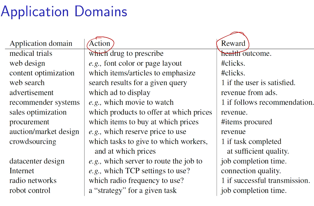
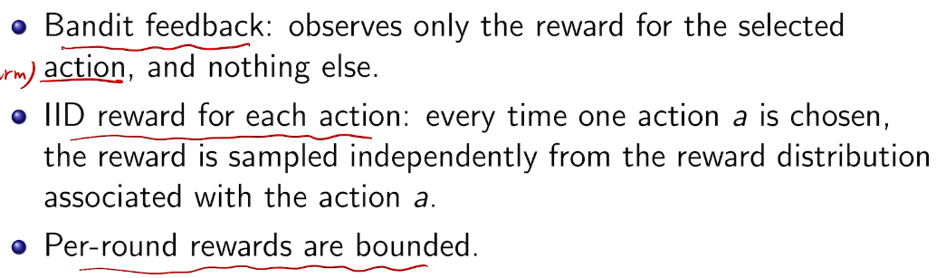
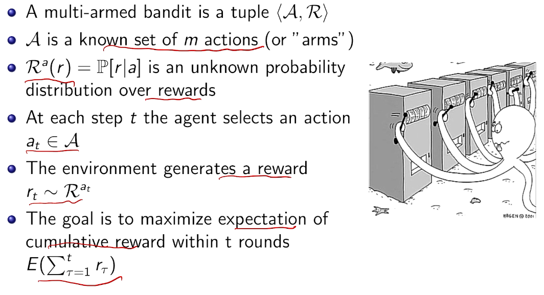
insights

  1. NF in awk is the number of fields divided by '/'! Not the number of '/'!
  2. After the '/' at the end of the line, even if there are no more characters, it is then counted into a field!
  3. For example, the following: drwxr-xr-x root / root 0 2011-08-26 09:18 bin / This is 3 fields! !! !!

CS 150 is composed of the TsingHua's 计算机组成原理 and VSLI

CS 150 is composed of the TsingHua's 计算机组成原理 and VSLI

source:http://www-inst.eecs.berkeley.edu/~cs150/sp13/agenda/

image-20200326172234625

They studied verilog

FSM is really similar to our homework. actually, I found that their exams is given to us for homework.

P.S.: WHY they have spring break?image-20200326172618489

image-20200326172816315

run a linux on FPGA. and implement a CPU. 俗称“造机”。

If I have time, I'll implement the CPU by my own.

GPU applying the RISC-V architecture will be much better and cooler.

The more I read and learn , the more I found the knowledge in the EECS category can be nicely cascaded. In most of the cases, we get the point from another place and we can be taught within minutes.

After talking with upperclassman 罗浩聪, I guadully find my career as an PhD in Arch or PL, or sth, in between. But for now, let me finish the 2 cooperate papers.

[Computer Architecture] Circuit

intro

image-20200325123544978

synchronous digital systems

Hardware of a processor should be synchronous and digital

The hardware layer of abstraction

image-20200325123706861

switches

image-20200325123737670

arrow shows action if wire changes to 1 or is asserted.

and & or

image-20200325123840940

Transistors

High voltage$V_{dd}$ Low voltage \(Gnd\)

PWD

we implement switches using CMOS

CMOS Transistor Networkimage-20200325124156574

image-20200325124245875vsimage-20200325124301345

note PWD

material:image-20200325124415901

how MOSFET Operation

image-20200325124509056
image-20200325124827736

CMOS Networks

2 input network

image-20200325141011777

combined logit symbols

image-20200325141058284

example debugging waveform

image-20200325140800590
image-20200325140219499

types of circuits

CL

SL

image-20200325140345618

example using time chart

image-20200325140122110

[RL] Bandit 算法

反馈:奖励

agent

action

image-20200323202634980

bandit 是强化学习的特例

利用与探索的两难

image-20200323201224285

短期与长期的对决

现实中的例子

image-20200323202023702

两臂老虎机

image-20200323202052208

三种类型

image-20200323201115089

奖励模型

image-20200323201147330

Decision making under uncertainty

image-20200323202734469

action vs. reward

image-20200323202834612

types of reward

image-20200323202956864

types of rewards model

image-20200323203015693

types of context

image-20200323203036389

example

image-20200323203050013

先验or后验

structured

global

summary

image-20200323203151320

example

网飞 展示广告

随机bandit

image-20200323203325042

image-20200323203342197

regret: equivalent goal

the value of an arbitrary action a is the mean reward for a (unknown):

image-20200323203438417

the optimal value is image-20200323203451851

we care about total regret

image-20200323203519243

image-20200323203526999

example on a

In general, those values are unknown.

we must try actions to learn the action-values(explore), and prefer those that appear best(exploit).

image-20200323203735348

action-value methods

image-20200323203817595

methods that learn action-value estimates and nothing else

根据强大数定理。收敛于真实期望值。

counting regret

image-20200323203927822

桥梁:计算total regret。 变量为指示变量

image-20200323204235802

image-20200323204326559image-20200323204347402

image-20200323204427181

亚当定理:得到lemma的结果

how to define a good learner.

image-20200323204604537

linear!! 有两种情况

image-20200323204646089

Greedy algorithm

image-20200323204721559

每次取最高的期望

\(\epsilon - greedy\)

防止出现局部最优

image-20200323204820675

proof of lower bound

image-20200323204836932

incremental implementation

性能考量、实现在线学习

image-20200323204942027

proof

image-20200323205150459

bandit notation

image-20200323205226555

image-20200323205237009

image-20200323205250785

进一步提高性能 Optimistic Initial values

All methods s ofar depends on image-20200323205414740 
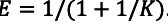
which is 0 in this case. but we can do 5.

Initally bad case for more 尝试。

image-20200323205430019

algorithm

image-20200323205543177

DecayIng \(\epsilon _{t} -Greedy\)

insight:先降后升

image-20200323205851377

performance comparison

image-20200323205925713## 
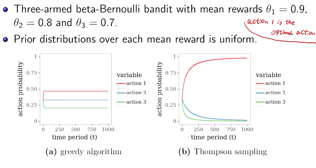
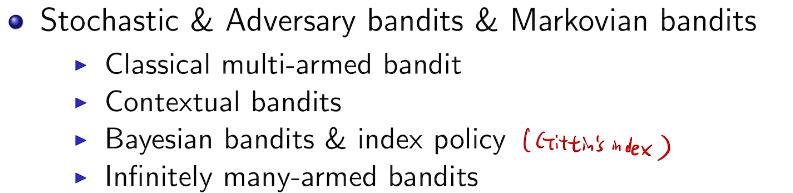
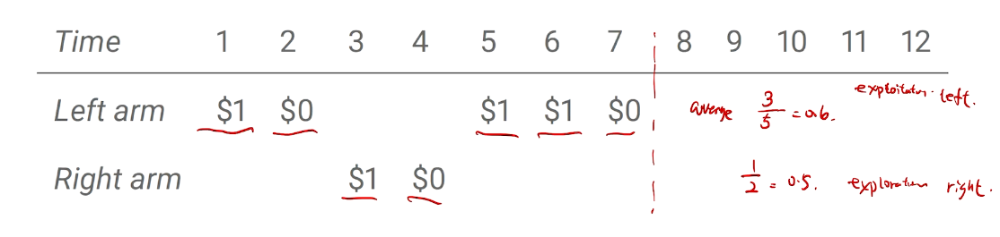
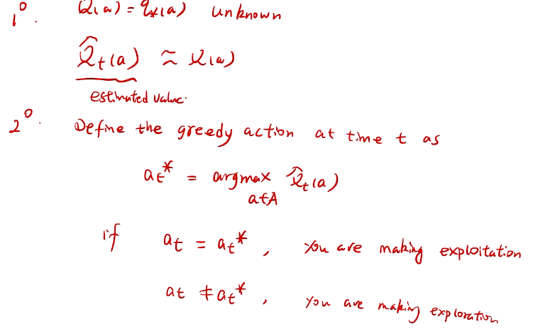
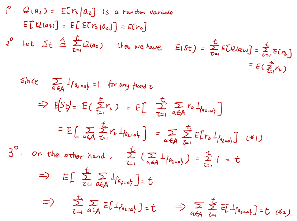
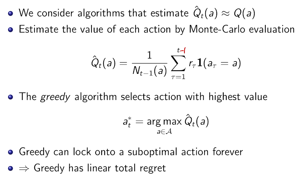
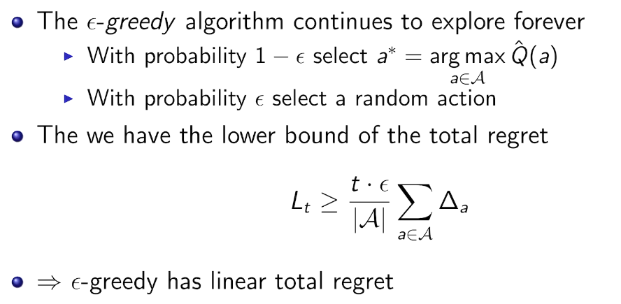
bandit algorithm lower bounds(depends on gaps)

image-20200323210003976

Optimism in the face of uncertainty

image-20200323210132650

which action to pick?

image-20200323210152032

越未知需要探索

Upper Confidence Bound

image-20200323210543776

hoeffding's inequality

image-20200323210628855

general case

image-20200323210645481

calculation

image-20200323210718913

取bound得到置信区间的位置

UCB1

image-20200323210818935

action 没有被充分的探索过,所以需要探索

上界探索

credit:https://jeremykun.com/2013/10/28/optimism-in-the-face-of-uncertainty-the-ucb1-algorithm/

Theorem: Suppose UCB1 is run as above. Then its expected cumulative regret \mathbb{E}(latex-1584977927119.png) 
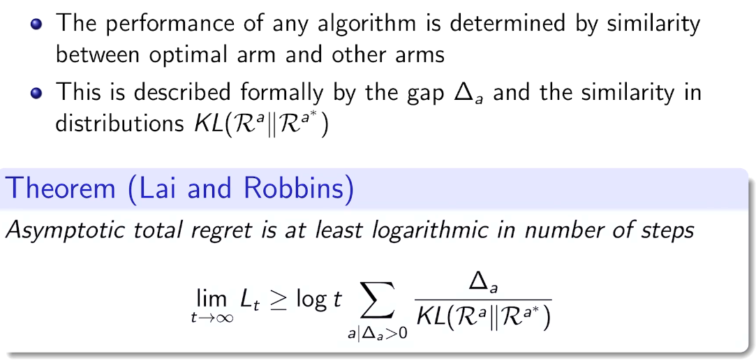
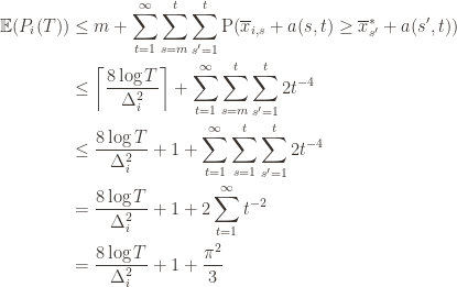
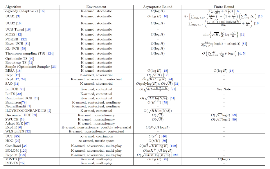
is at most$\displaystyle 8 \sum_{i : \mu_i < \mu^*} \frac{\log T}{\Delta_i} + \left ( 1 + \frac{\pi^2}{3} \right ) \left ( \sum_{j=1}^K \Delta_j \right )$

Okay, this looks like one nasty puppy, but it’s actually not that bad. The first term of the sum signifies that we expect to play any suboptimal machine about a logarithmic number of times, roughly scaled by how hard it is to distinguish from the optimal machine. That is, if \Delta_i is small we will require more tries to know that action i is suboptimal, and hence we will incur more regret. The second term represents a small constant number (the $1 + \pi^2 / 3$ part) that caps the number of times we’ll play suboptimal machines in excess of the first term due to unlikely events occurring. So the first term is like our expected losses, and the second is our risk.

But note that this is a worst-case bound on the regret. We’re not saying we will achieve this much regret, or anywhere near it, but that UCB1 simply cannot do worse than this. Our hope is that in practice UCB1 performs much better.

Before we prove the theorem, let’s see how derive the O(latex-1584977927114.png) 
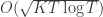
bound mentioned above. This will require familiarity with multivariable calculus, but such things must be endured like ripping off a band-aid. First consider the regret as a function R(latex-1584977927125.png) (excluding of course \Delta^*), and let’s look at the worst case bound by maximizing it. In particular, we’re just finding the problem with the parameters which screw our bound as badly as possible, The gradient of the regret function is given by

\displaystyle \frac{\partial R}{\partial \Delta_i} = - \frac{8 \log T}{\Delta_i2} + 1 + \frac{\pi2}{3}

and it’s zero if and only if for each i, } = O(latex-1584977927124.png). However this is a minimum of the regret bound (the Hessian is diagonal and all its eigenvalues are positive). Plugging in the \Delta_i = O(latex-1584977927170.png) 
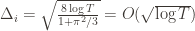
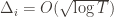
(which are all the same) gives a total bound of O(latex-1584977927132.png). If we look at the only possible endpoint (the \Delta_i = 1), then we get a local maximum of O(latex-1584977927132.png). But this isn’t the O(latex-1584977927114.png) we promised, what gives? Well, this upper bound grows arbitrarily large as the \Delta_i 
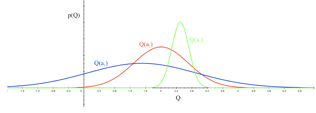
go to zero. But at the same time, if all the \Delta_i are small, then we shouldn’t be incurring much regret because we’ll be picking actions that are close to optimal!

Indeed, if we assume for simplicity that all the \Delta_i = \Delta are the same, then another trivial regret bound is \Delta T (why?). The true regret is hence the minimum of this regret bound and the UCB1 regret bound: as the UCB1 bound degrades we will eventually switch to the simpler bound. That will be a non-differentiable switch (and hence a critical point) and it occurs at \Delta = O(latex-1584977927136.png)
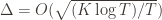
. Hence the regret bound at the switch is \Delta T = O(latex-1584977927304.png), as desired.

Proving the Worst-Case Regret Bound

Proof. The proof works by finding a bound on P_i(latex-1584978965148.png)
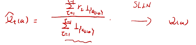
, the expected number of times UCB chooses an action up to round T. Using the \Delta 
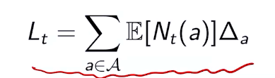
notation, the regret is then just \sum_i \Delta_i \mathbb{E}(latex-1584978965117.png), and bounding the P_i‘s will bound the regret.

Recall the notation for our upper bound a(latex-1584978965147.png) = \sqrt{2 \log T / P_j(T)} and let’s loosen it a bit to a(latex-1584978965148.png) = \sqrt{2 \log T / y} so that we’re allowed to “pretend” a action has been played y times. Recall further that the random variable I_t 
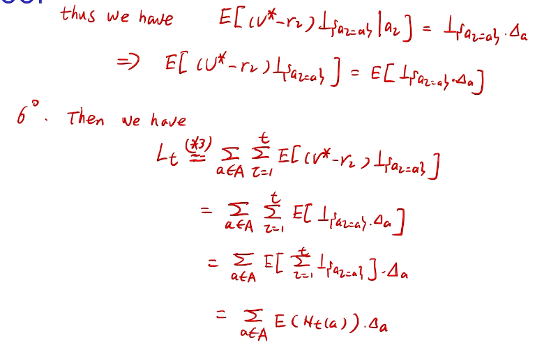
has as its value the index of the machine chosen. We denote by \chi(latex-1584978965127.png) the indicator random variable for the event E. And remember that we use an asterisk to denote a quantity associated with the optimal action (e.g., \overline{x}^* is the empirical mean of the optimal action).

Indeed for any action i, the only way we know how to write down P_i(T) is as

\displaystyle P_i(latex-1584978965149.png) = 1 + \sum_{t=K}^T \chi(I_t = i)

The 1 is from the initialization where we play each action once, and the sum is the trivial thing where just count the number of rounds in which we pick action i. Now we’re just going to pull some number m-1 of plays out of that summation, keep it variable, and try to optimize over it. Since we might play the action fewer than m times overall, this requires an inequality.

P_i(latex-1584978965206.png) \leq m + \sum_{t=K}^T \chi(I_t = i \textup{ and } P_i(t-1) \geq m)

These indicator functions should be read as sentences: we’re just saying that we’re picking action i in round t and we’ve already played i at least m times. Now we’re going to focus on the inside of the summation, and come up with an event that happens at least as frequently as this one to get an upper bound. Specifically, saying that we’ve picked action i in round t means that the upper bound for action i exceeds the upper bound for every other action. In particular, this means its upper bound exceeds the upper bound of the best action (and i might coincide with the best action, but that’s fine). In notation this event is

\displaystyle \overline{x}_i + a(latex-1584978965271.png) \geq \overline{x}* + a(P*(T), t-1)

Denote the upper bound \overline{x}_i + a(latex-1584978965272.png) for action i in round t by U_i(latex-1584978965333.png). Since this event must occur every time we pick action i (though not necessarily vice versa), we have

\displaystyle P_i(latex-1584978964873.png) \leq m + \sum_{t=K}T \chi(U_i(t-1) \geq U*(t-1) \textup{ and } P_i(t-1) \geq m)

We’ll do this process again but with a slightly more complicated event. If the upper bound of action i exceeds that of the optimal machine, it is also the case that the maximum upper bound for action i we’ve seen after the first m trials exceeds the minimum upper bound we’ve seen on the optimal machine (ever). But on round t we don’t know how many times we’ve played the optimal machine, nor do we even know how many times we’ve played machine i (except that it’s more than m). So we try all possibilities and look at minima and maxima. This is a pretty crude approximation, but it will allow us to write things in a nicer form.

Denote by \overline{x}_{i,s} the random variable for the empirical mean after playing action i a total of s times, and \overline{x}^*_s the corresponding quantity for the optimal machine. Realizing everything in notation, the above argument proves that

\displaystyle P_i(T) \leq m + \sum_{t=K}T \chi \left ( \max_{m \leq s < t} \overline{x}{i,s} + a(s, t-1) \geq \min{0 < s' < t} \overline{x}*_{s'} + a(s', t-1) \right )

Indeed, at each t for which the max is greater than the min, there will be at least one pair s,s' for which the values of the quantities inside the max/min will satisfy the inequality. And so, even worse, we can just count the number of pairs s, s' for which it happens. That is, we can expand the event above into the double sum which is at least as large:
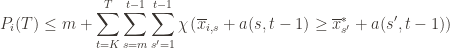
\displaystyle P_i(T) \leq m + \sum_{t=K}T \sum_{s = m}{t-1} \sum_{s' = 1}{t-1} \chi \left ( \overline{x}_{i,s} + a(s, t-1) \geq \overline{x}*_{s'} + a(s', t-1) \right )

We can make one other odd inequality by increasing the sum to go from t=1 to \infty
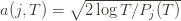
. This will become clear later, but it means we can replace t-1 with t and thus have

\displaystyle P_i(T) \leq m + \sum_{t=1}\infty \sum_{s = m}{t-1} \sum_{s' = 1}{t-1} \chi \left ( \overline{x}_{i,s} + a(s, t) \geq \overline{x}*_{s'} + a(s', t) \right )

Now that we’ve slogged through this mess of inequalities, we can actually get to the heart of the argument. Suppose that this event actually happens, that \overline{x}{i,s} + a(s, t) \geq \overline{x}^*{s'} + a(s', t). Then what can we say? Well, consider the following three events:

(1) \displaystyle \overline{x}*_{s'} \leq \mu* - a(s', t)
(2) \displaystyle \overline{x}_{i,s} \geq \mu_i + a(latex-1584978965039.png)
(3) \displaystyle \mu^* < \mu_i + 2a(s, t)

In words, (1) is the event that the empirical mean of the optimal action is less than the lower confidence bound. By our Chernoff bound argument earlier, this happens with probability t^{-4}
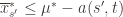
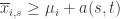
. Likewise, (2) is the event that the empirical mean payoff of action i is larger than the upper confidence bound, which also occurs with probability t^{-4}. We will see momentarily that (3) is impossible for a well-chosen m (which is why we left it variable), but in any case the claim is that one of these three events must occur. For if they are all false, we have

\displaystyle \begin{matrix} \overline{x}{i,s} + a(s, t) \geq \overline{x}^*{s'} + a(s', t) & > & \mu^* - a(s',t) + a(s',t) = \mu^* \ \textup{assumed} & (1) \textup{ is false} & \ \end{matrix}

and

\begin{matrix} \mu_i + 2a(s,t) & > & \overline{x}{i,s} + a(s, t) \geq \overline{x}^*{s'} + a(s', t) \ & (2) \textup{ is false} & \textup{assumed} \ \end{matrix}

But putting these two inequalities together gives us precisely that (3) is true:

\mu^* < \mu_i + 2a(s,t)

This proves the claim.

By the union bound, the probability that at least one of these events happens is 2t^{-4} plus whatever the probability of (3) being true is. But as we said, we’ll pick m to make (3) always false. Indeed m depends on which action i is being played, and if
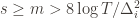
 s \geq m > 8 \log T / \Delta_i^2 then 2a(latex-1584978965191.png) \leq \Delta_i, and by the definition of \Delta_i we have

\mu^* - \mu_i - 2a(latex-1584978965195.png) \geq \mu^* - \mu_i - \Delta_i = 0.

Now we can finally piece everything together. The expected value of an event is just its probability of occurring, and so

\displaystyle \begin{aligned} \mathbb{E}(P_i(T)) & \leq m + \sum_{t=1}\infty \sum_{s=m}t \sum_{s' = 1}t \textup{P}(\overline{x}_{i,s} + a(s, t) \geq \overline{x}*_{s'} + a(s', t)) \ & \leq \left \lceil \frac{8 \log T}{\Delta_i2} \right \rceil + \sum_{t=1}\infty \sum_{s=m}t \sum_{s' = 1}t 2t{-4} \ & \leq \frac{8 \log T}{\Delta_i2} + 1 + \sum_{t=1}\infty \sum_{s=1}t \sum_{s' = 1}t 2t{-4} \ & = \frac{8 \log T}{\Delta_i2} + 1 + 2 \sum_{t=1}\infty t^{-2} \ & = \frac{8 \log T}{\Delta_i2} + 1 + \frac{\pi2}{3} \ \end{aligned}

The second line is the Chernoff bound we argued above, the third and fourth lines are relatively obvious algebraic manipulations, and the last equality uses the classic solution to Basel’s problem. Plugging this upper bound in to the regret formula we gave in the first paragraph of the proof establishes the bound and proves the theorem.

result

image-20200324001226338

Intro for Thompson Sampling

Probability Matching

image-20200324001312794

~ 最大后验概率

image-20200324001334684

history

image-20200324001445661

在知道后验的情况下比UCB 好

beta-bernoulli bandit

image-20200324001641824

先验共轭

image-20200324001710568

greedy vs. Thompson Sampling

image-20200324001741847

第一步不一样。 期望 vs 样本值

simulation

image-20200324001834578

image-20200324001902205

image-20200324001918590

Other kind of Bayesian inference

image-20200324002105541

梯度bandit 算法

随机梯度上升法

image-20200324002149133

image-20200324002430374

why not 梯度下降?

​ more general for RL

image-20200324002556856

proof

image-20200324004923787

image-20200324005138180

// lemma 1 for homework

image-20200324005203636

image-20200324005337331

image-20200324005415850

image-20200324005443234

梯度的期望->期望的梯度

Adversarial Bandit

image-20200324005708760

simple bandit game

image-20200324005804371

image-20200324010052550

importance-weighted estimators

image-20200324010145087

用于估计其他未被触发的arm

another good algorithm

image-20200324011008118

bias ~ variance tradeoff

方差太大。

几率小的reward 现在增大了。 用隐含的增加的探索来使反差减少

algorithm

image-20200324011146738

adversary bandits with expert's advice

image-20200324011216181

image-20200324011302481

意见的权重的分布=》exp4

additional exploration

uniform exploration

proved no need

image-20200324011420766

summary

image-20200324011450638

bound

image-20200324011524504

看作为独立为RL之外的眼界方向

image-20200324011616176

[Parallel Computing] Implementing collective communication

Collective communication

  • Important as the basis for many parallel algorithms.
  • Implemented using multiple point to point communications, possibly in parallel.
    • Assume communicating m words (without contention) between a source and destination takes \(t_{s} + m t_{w}\) time.
    • Ignore the the distance of the message, since per hop latency th is usually small.
  • With contention c, time becomes \(t_{s} + c m t_{w}\).
  • Implementations depend on communication hardware architecture.
  • Operations
  • Broadcast and reduction.
  • All-to-all broadcast and reduction.
  • All-reduce, prefix sum.
  • Scatter and gather.
  • All-to-all scatter and reduce.
  • Circular shift.

Broadcast and reduction on ring

image-20200323151043402

just cut them into halves.

cost

  • With p processors, log p steps.
  • In each step, a processor sends a size m message.
  • Total time$ (t_{s} + m t_{w}) log p$ take \((t_{s} + m t_{w})\) as const

Broadcast on mesh

image-20200323152756914

algorithm

  • Root first broadcasts along its row using ring algorithm.
  • The nodes of root’s row then broadcast along their columns using ring algorithm.

cost

  • \(log \sqrt{p} = (log p) / 2\) steps along row, same along columns.
  • Total time (ts + m tw) log p.log
  • p = (log p) / 2 steps along row, same along columns.
  • Total time (ts + m tw) log p.

Broadcast on hypercube

algorithm

image-20200323151732584

RING CAN BE PROJECTED TO THE HYPERCUBE but with more congestion.

prefix sum on hypercube

image-20200323154823396

[Computer Architechture] call

Language Execution continuum

An interpreter is a program that executes other programs.

  1. langurage translation gives us another option
  2. In genreral, we interpret a high-level language to a lower-level language to increase preformance

image-20200320143508476

interpretation

  1. Python
  2. asm

Assembler directives

image-20200320143656584

pseudo-instruction replacement

image-20200320143736406

what's tail's about
{...
 lots of code
 return foo(y);
}
  • it's recursive call to foo() if this is within foo(), or call to a different function...
  • for effictiency
    • Evaluate the arguments for foo() in a0-a7
    • return ra, all callee saved registers and sp
    • Then call foo() with j or tail
  • when foo() returns, it can return directly to where it needs to return to
    • Rather than returning to wherever foo() was called and returning from there
    • Tail call optimization

branches

image-20200320144520209

Linking progress

image-20200320150133861

image-20200320150156550

Four types of Address

PC- relative addredding (beq)

Absolute addresses in RISC-V

image-20200320150357128

Loading process

image-20200320150929601

Running a Program - CALL(Compiling, Assembling, Linking, and Loading)

Clarifications

Project 1 RISC-v emulator

  1. Risc-v isa does not define assembly syntax
    behave exactly like Venus
  2. All I-Type instructions (including sltiu)
    • do sign-extension
    • (in venus) input number is signed, even if hex

a good tool

Interpretation

  1. any good reason to interpret machine language in software? debbuger Venus
  2. translated/compiled code almost always more efficitent and therfore higher performance:
    • important for many applications, particularly operating systems.

Steps in compiling a C program

Psuedo-instruciton Replacement

Producing Machine Language

  • simple case
    • arithmetic, logical, shifts and so on
    • All necessary info is within the instruction already
  • branches can be optimized

parallel programing 23 parallel fft

One of the most import algorithm in the new century

Intro to the fft

The basic equation of the FFT

\(F(\omega)=F|f(t)|=\int ^{+\infty}_{-\infty}f(t)e^{-j\omega t}dt\)

Roots of unity

\[
\begin{array}{l}\text { An n'th root of unity is an } \omega \text { s.t. } \ \omega^{n}=1 \text { . } \ \text { There are n roots n'th roots of } \ \text { unity, and they have the form } \ e^{\frac{2 \pi i k}{n}}, \text { for } 0 \leq k \leq n-1 \text { . } \ \text {Write } \omega_{n}=e^{\frac{2 \pi i}{n}} \text { , so that the n'th } \ \text { roots of unity are } \omega_{n}^{0}, \omega_{n}^{1}, \ldots, \omega_{n}^{n-1} \end{array}\]

Some problems to differ DT,DFT,FFT,IFFT

They are Fourier Transform, Discrete Fourier Transform, Fast Fourier Transform and Inverse Fourier Transform.
The transform factor:
\(\text { Fact } 1 \omega_{n}^{n}=1 \text { . } \ \text { Fact } 2 \omega_{n}^{k+\frac{n}{2}}=-\omega_{n}^{k} \ \text { Fact } 3\left(\omega_{n}^{k}\right)^{2}=\omega_{n}^{2 k}=\omega_{n / 2}^{k}\)

Why we should have the DFT.
Because in theory, all the data stored in computer is Discrete. So we have to use the equation \(X(k)=\sum^{N-1}_0x(n)W^{kn}_N(k\in \mathbb{N})\)

The Transform factor is used to prove the
1) Periodicity
\(W_{N}^{m+l N}=W_{N}^{m},\)\) where \(\(: W_{N}^{-m}=W_{N}^{N-m}\)
2) Symmetry
\(W_{N}^{m+\frac{N}{2}}=-W_{N}^{m}\)
3) Contractability
\(W_{N / m}^{k}=W_{N}^{m k}\)
4) Special rotation factors
\(W_{N}^{0}=1\)

  1. Why Fourier Fast Algorithm (aka FFT)?

FFT is a DFT-based algorithm designed to accelerate the computational speed of DFT.

Given a degree \(n\) -1 polynomial
\(A(x)=a_{0}+a_{1} x+a_{2} x^{2}+\dots+a_{n-1} x^{n-1}\)
DFT computes \(A\left(\omega_{n}^{0}\right), A\left(\omega_{n}^{1}\right), \ldots, A\left(\omega_{n}^{n-1}\right)\)
since \(A(x)=a_{0}+x\left(a_{1}+x\left(a_{2}+\cdots\right) \ldots\right)\)
\(A(x)\) can be evaluated in \(\mathrm{O}(\mathrm{n})\) time and
\(\mathrm{O}(1)\) memory.

  • DFT can be computed trivially in \(\mathrm{O}\left(\mathrm{n}^{2}\right)\)
    time.

For the DFT formula computer implementation the complexity is o(N²), while the complexity by FFT calculation is reduced to: N×log2(N)

  1. What is the sequence split extraction in FFT?

The sequence splitting process of FFT is the extraction process, which is divided into: extraction by time and extraction by frequency.

1) Extraction by time (also called parity extraction)


2) Frequency, which we don’t apply here.

  1. How does FFT reduce the amount of computation?

In simple terms, mathematicians use the above mentioned properties of the rotation factor W such as periodicity, symmetry, etc. to simplify the formula. In algorithmic programming, new points are constantly counted using points that have already been counted, i.e., old points count new points.

Theoretically, FFT computes the DFT in O(n log n) time using divide and conquer.
\square Suppose n is a power of 2.
Let \(A^{[0]}=a_{0}+a_{2} x^{1}+a_{4} x^{2}+\cdots+a_{n-2} x^{\frac{n}{2}-1}\)
\(A^{[1]}=a_{1}+a_{3} x^{1}+a_{5} x^{2}+\cdots+a_{n-1} x^{\frac{n}{2}-1}\)
Then \(A(x)=A^{[0]}\left(x^{2}\right)+x A^{[1]}\left(x^{2}\right)\).
So can compute \(A\left(\omega_{n}^{0}\right), A\left(\omega_{n}^{1}\right), \ldots, A\left(\omega_{n}^{n-1}\right)\) by computing \(A^{[0]}\) and \(A^{[1]}\)
at \(\left(\omega_{n}^{0}\right)^{2},\left(\omega_{n}^{1}\right)^{2}, \ldots,\left(\omega_{n}^{n-1}\right)^{2}\), and multiplying some terms by
\(\omega_{n}^{0}, \omega_{n}^{1}, \ldots, \omega_{n}^{n-1}\).
But \(\left(\omega_{n}^{k+n / 2}\right)^{2}=\omega_{n}^{2 k+n}=\omega_{n}^{2 k}=\left(\omega_{n}^{k}\right)^{2}\) by Fact 1.
A So \(\left\{\left(\omega_{n}^{0}\right)^{2},\left(\omega_{n}^{1}\right)^{2}, \ldots,\left(\omega_{n}^{n-1}\right)^{2}\right\}=\left\{\left(\omega_{n}^{0}\right)^{2},\left(\omega_{n}^{1}\right)^{2}, \ldots,\left(\omega_{n}^{n / 2-1}\right)^{2}\right\},\) i.e. only need
to evaluate \(A^{[0]}\) and \(A^{[1]}\) at n/2 points instead of n.
Also, \(\left(\omega_{n}^{k}\right)^{2}=\omega_{n}^{2 k}=\omega_{n / 2}^{k}\)

Note: Simply splitting a multipoint sequence into a less point sequence without simplification is not a reduction in arithmetic volume!!! Splitting is only in the service of simplification, using the spin factor is the key to arithmetic reduction!!!

Time Complexity:
Thus, computing \(A(x)=A^{[0]}\left(x^{2}\right)+x A^{[1]}\left(x^{2}\right)\) for
\(x \in\left\{\omega_{n}^{0}, \omega_{n}^{1}, \ldots, \omega_{n}^{n-1}\right\}\) requires
\(\square\) Computing for \(A^{[0]}(x)\) and \(A^{[1]}(x)\) for \(x \in\)
\(\left\{\omega_{n / 2}^{0}, \omega_{n / 2}^{1}, \ldots, \omega_{n / 2}^{n / 2-1}\right\}\)

  • These are also DFT’s, so can be done recursively using two
    n/2-point FFT’s.
    \square For \(0 \leq k \leq \frac{n}{2}-1\)
    \[
    \begin{array}{l}\qquad A\left(\omega_{n}^{k}\right)=A^{[0]}\left(\omega_{n / 2}^{k}\right)+\omega_{n}^{k} A^{[1]}\left(\omega_{n / 2}^{k}\right) \ \begin{array}{l}\qquad A\left(\omega_{n}^{k+n / 2}\right)=A^{[0]}\left(\omega_{n / 2}^{k+n / 2}\right)+\omega_{n}^{k+n / 2} A^{[1]}\left(\omega_{n / 2}^{k+n / 2}\right) \ =A^{[0]}\left(\omega_{n / 2}^{k}\right)-\omega_{n}^{k} A^{[1]}\left(\omega_{n / 2}^{k}\right)\end{array}\end{array}
    \]

  1. Butterfly operation?

For a butterfly operation, you can understand it as an operation that is customizable by a graph.

The left side is the input and the right side is the output, for the letters on the horizontal line there are two cases.

1) A number on the left end line (none means C and D are 1).

2)The right end lines have the numerical representation, but if none, C & D are 0s.

The FFT takes out odd and even in accordance to time to change the original sequence. which have to sequentialize it to make the algorithm meet the required sequence. The new sequence is the reverse binary sequence of the original ones.

For example \((a_0 a_4 a_2 a_6 a_1 a_5 a_3 a_7)\) have the binary sequence \((000,100,010,110,001,101,011,111)\).
The reverse order can be simply treated as the change of 2 near binary number, which in this case is:\((a_0 a_1 a_2 a_3 a_4 a_5 a_6 a_7)\);

Which is \((000,001,010,011,100,101,110,111)—>(000,100,010,110,001,101,011,111)\).

The code for this transformation:

for(I=0;I<N;I++) // According to law 4, you need to perform inter-code inverse order for all elements of the array
{  
  /* Get the value of the inverse J of subscript I*/ 
  J=0;
  for(k=0;k<(M/2+0.5);k++) //k indicates operation
     {
        /* Reverse sequence operation*/
        m=1;//m is a binary number with a minimum of 1
        n=(unsigned int)pow(2,M-1);//n is a binary number with the Mth degree of 1.
        m <<= k; // for m move left k
        n>>= k; //shift k bits to the right of n
        F0=I & n;//I & n by the kth position of the first half of the extracted
        F1=I & m;//I with m-pressure bit corresponding to the lower part of the second half of the extracted F0
        if(F0) J=J | m; //J and m are in position or so that F0 corresponds to a low position of 1
        if(F1) J=J | n; //J and n are in the same position or so that F1 corresponds to a high level of 1
     }
   if(I<J)
    {
      Temp=A[I];
      A[I] =A[J];
      A[J]=Temp;
    }                                
}

The butter fly operation:
Now let’s imagine that if we want to program the FFT algorithm, the most basic implementation of the FFT algorithm is the butterfly operation, for any butterfly such as.

When N=8.

As can be seen from the above figure, to perform the butterfly operation, we have to solve the following problems.

  • Interval B between two input data

  • Determination of the rotation factor W, including.

    • Determination of the L-level rotation index P.
    • Determination of the type of Level L W.
    • The interval between the same W in level L.

\(\left\{\begin{array}{l}T_{R}=X_{R}(\mathrm{j}+B) \cos \frac{2 \pi}{N} p+X_{I}(j+B) \sin \frac{2 \pi}{N} p \cdots(1) \ T_{\mathrm{I}}=X_{I}(j+B) \cos \frac{2 \pi}{N} p-X_{R}(j+B) \sin \frac{2 \pi}{N} p \cdots(2) \ \mathrm{A}_{\mathrm{R}}(\mathrm{j})=X_{R}(\mathrm{j})+T_{R} \ \mathrm{A}_{\mathrm{I}}(\mathrm{j})=X_{I}(\mathrm{j})+T_{\mathrm{I}} \ \mathrm{A}_{\mathrm{R}}(\mathrm{j}+\mathrm{B})=X_{R}(\mathrm{j})-T_{R}(5) \ \mathrm{A}_{\mathrm{I}}(\mathrm{j}+\mathrm{B})=X_{I}(\mathrm{j})-T_{\mathrm{I}}(6)\end{array}\right.\)

for(L=1; L<=M;L++) //FFT butterfly level L from 1--M
{  
  /* L-level operations*/  
  //First calculate the interval B = 2^(L-1);
  B = 1;
  B = (int)pow(2,L-1);
  for(j=0; j<=B-1;j++)
  {
    /* Homogeneous butterfly operation*/  
    // First increment k=2^(M-L)
    k = (int)pow(2,M-L);
    // Calculate the rotation index p in increments of k, then p = j*k
    P=1;
    P=j*k;
    for(i=0; i<=k-1;i++)
    {
      /* Perform butterfly operations*/
      //Array calibrated to r
      r=1;
      r=j+2*B*i;
      Tr=dataR[r+B]*cos(2.0*PI*p/N) + dataI[r+B]*sin(2.0*PI*p/N);
      Ti=dataI[r+B]*cos(2.0*PI*p/N) - dataR[r+B]*sin(2.0*PI*p/N);
      dataR[r+B]=dataR[r]-Tr;
      dataI[r+B]=dataI[r]-Ti;
      dataR[r]=dataR[r]-Tr; dataI[r+B]=dataI[r]-Ti; dataI[r]-Ti; dataR[r]=dataR[r]+Tr;
      dataI[r]=dataI[r]]+Ti;
    }
  }
}

IFFT is the reverse of the above operation.

  1. What if we take it on the mesh or hypercube to make it scalable on gpu oprations?

Hpercube:

  • Consider the binary exchange algorithm on a hypercube architecture.
  • Each processor connected to d others, which differ in each digit of ID.
    • Communication only with neighbors, send n/p values each time.
    • since d = log p rounds of communication, communication time \(T_{c}=\) \(t_{s} \log p+t_{w} \frac{7}{p} \log p .\)
  • Each stage does n/p computation.
    • Total computation time \(T_{p}=\frac{t_{c} n}{p} \log n\).
  • Efficiency is \(E=\frac{T_{p}}{T_{p}+T_{c}}=1 /\left(1+\frac{t_{s} p \log p}{t_{c} n \log n}+\frac{t_{w} \log p}{t_{c} \log n}\right)\)
  • Define \(K\) such that \(E=1 /(1+1 / K) .\)
  • For isoefficiency, want last two terms in denominator to be constant.
  • \(\frac{t_{s} p \log p}{t_{c} n \log n}=\frac{1}{K}\) implies \(n \log n=W=K \frac{t_{s}}{t_{c}} p \log p .\)
  • \(\frac{t_{w} \log p}{t_{c} \log n}=\frac{1}{K}\) implies \(\log n=K_{t_{c}}^{t_{w}} \log p,\) so \(n=p^{K t_{w} / t_{c}},\) so
  • \(W=K \frac{t_{w}}{t_{c}} p^{K t_{w} / t_{c}} \log p\)

The efficiency for this case depends on \(t_c,t_s,t_w\), the wait time is the tradeoffs between two different lines. which is:

From the Efficiency law
, we have once \(\frac{Kt_w}{t_c}>1\), the increasing time is polynomial with regard to the processor count.

Mese:

2D transpose FFT: The best:

Reference

  1. Prof Fan’s PPT
  2. Implement FFT in C by GoKing
  3. Implement FFT on QPU rpi3b+ by Andrew Holme

Some invitation with ICE Zhang @Pennstate

Good to see that the emerging youngsters of Generation Z in China. When it comes to the Zhihu Question "What are 00s anxious about?" ICE Zhang points out a variety of great people. My answer was OIer, IMOer and those who have a lot of time digging one single target without any interference will temporarily take up the "bill board". But with time, people will get to realize this world need hero, a person who can see through the greatest evolution of the world and provide surging advise.

Zhang maybe that kind of person. I would say it's really hard to invite such a guy to Shanghai. But hopefully, he has a great amount of Gay Joy in Shanghai, mostly PingCap employees and his friends and his friends's friends in minority. I would say, before my internship, I never jump into the networking with strangers. But I found it funny. I dived into Persistent Memory stuff which is ideal for me. One man does not build the Rome. I need others' info and their progress to push myself. Only through others' progress can see my limit and inability and lack of determination.

I'm informed that the gay with ICE yesterday was even not enter her adulthood. The Turing Award Winner compose his poem at early 20s. I would say, I start late and I don't think I could dig as far as her. I'm a poor Math guy, even may fail at Daniel's Abstract Mathematic. I could have been captivated by Group, Ring and Field. I could have made systematic view of analysis and geometry. I could have write more elegant code to let other people endorse type theory. I can not because I've got only one body and one stream of mind.

I'm in favor of pursuing my own heart more. I find myself limited time in this place. I have to make all the stuff come true!