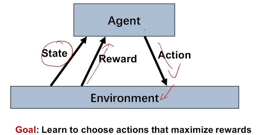
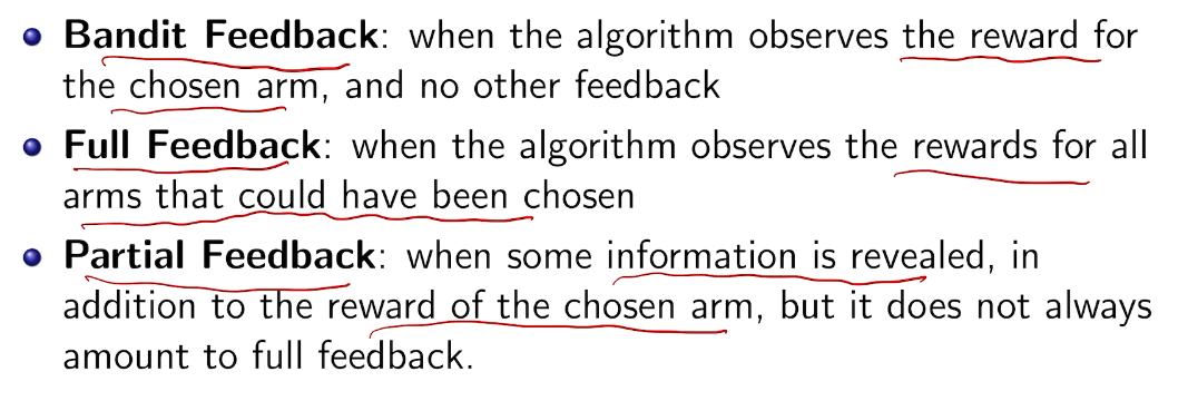
反馈:奖励
agent
action
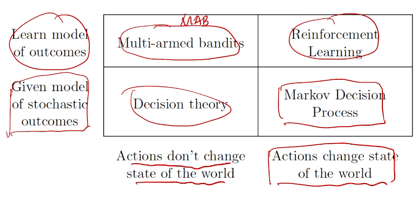
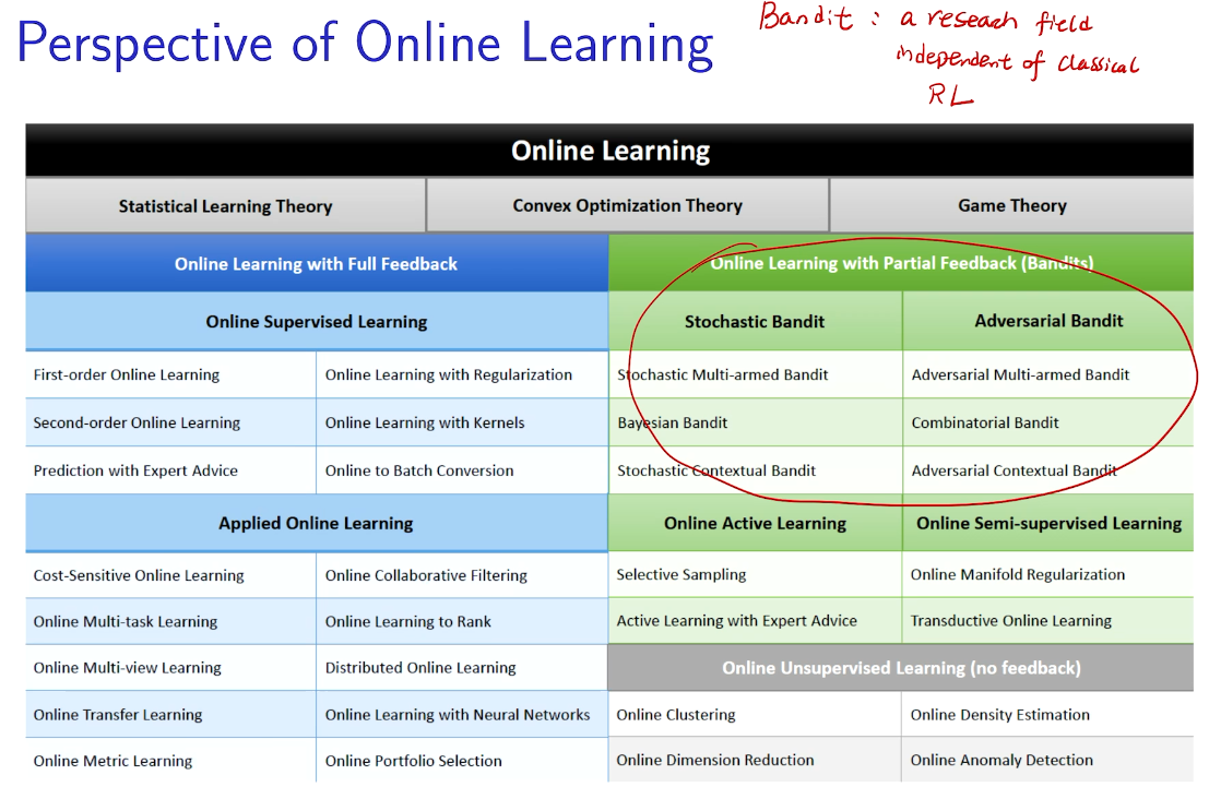
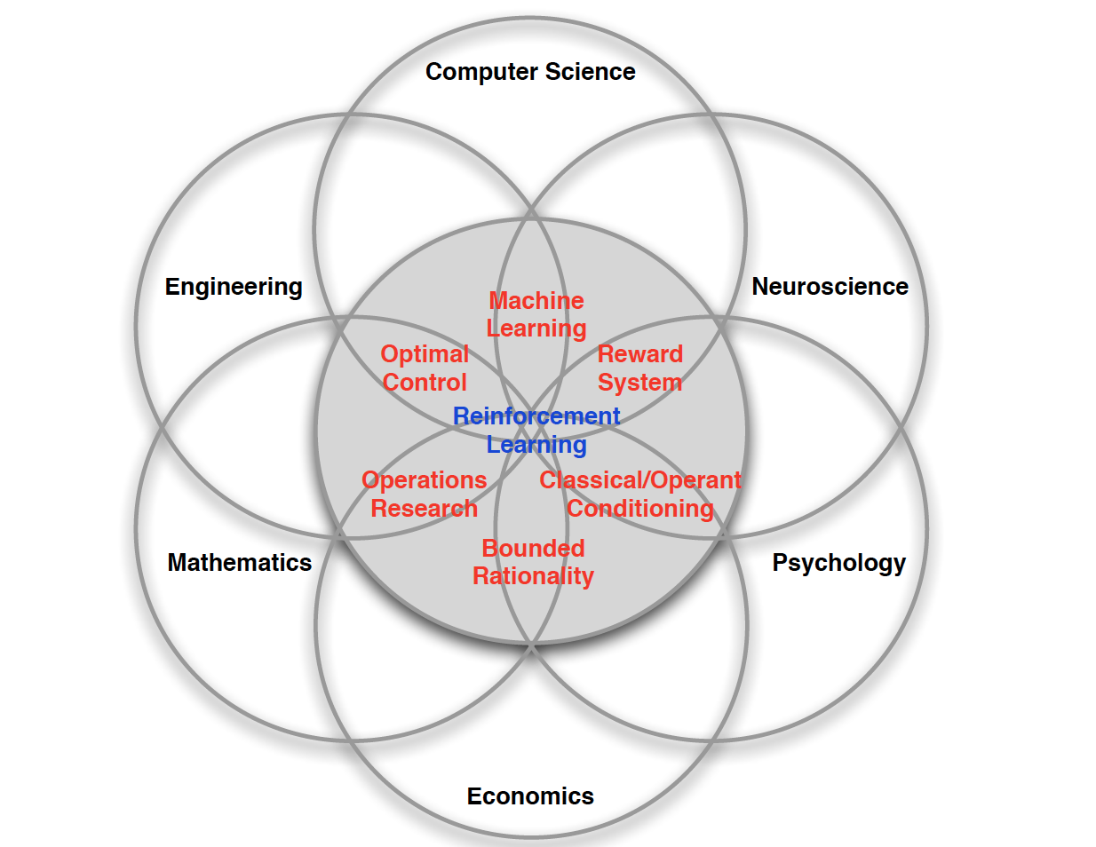
bandit 是强化学习的特例
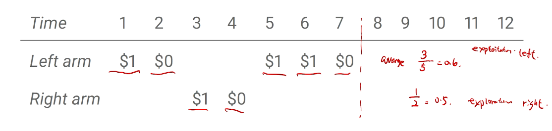
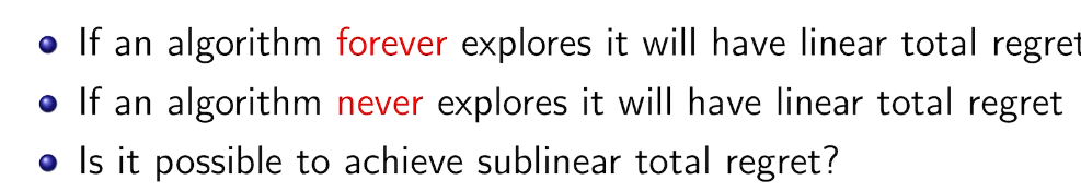
利用与探索的两难
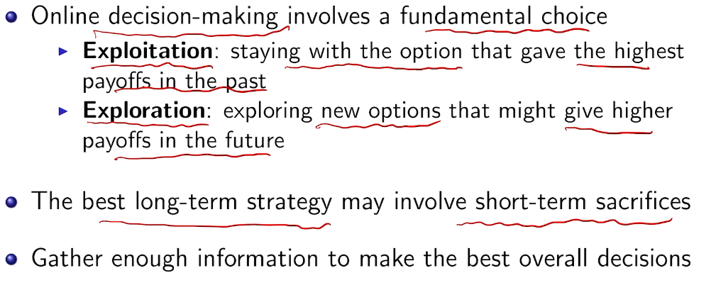
短期与长期的对决
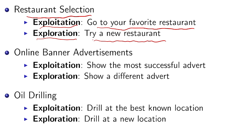
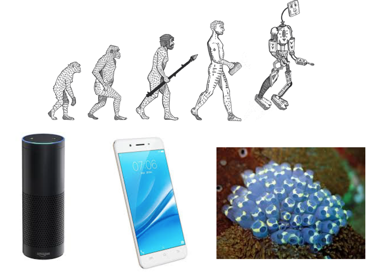
现实中的例子
两臂老虎机
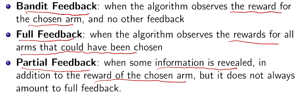
三种类型
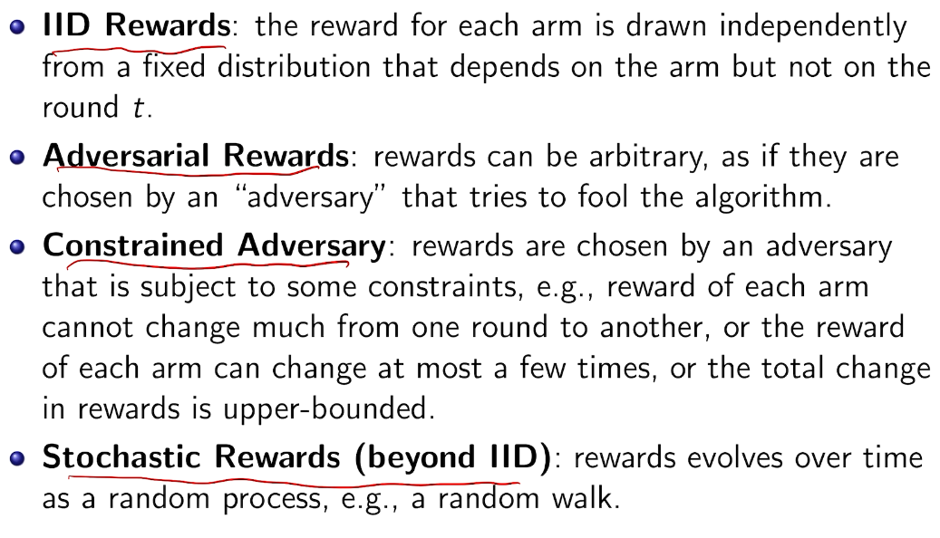
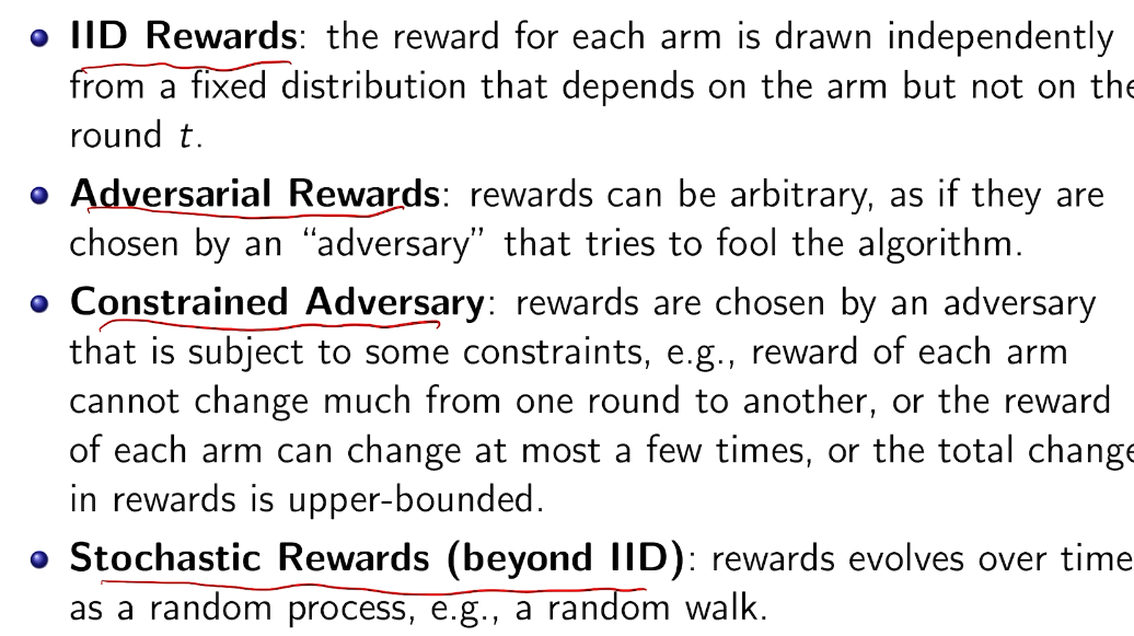
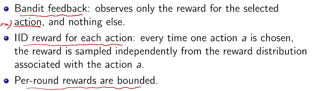
奖励模型
Decision making under uncertainty
action vs. reward
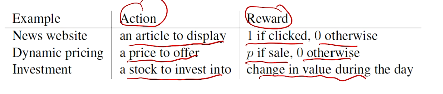
types of reward
types of rewards model
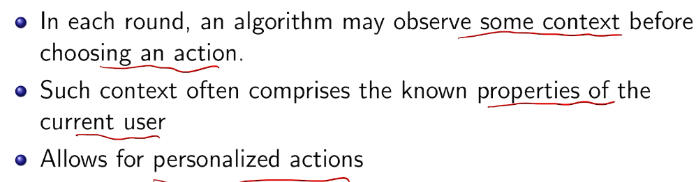
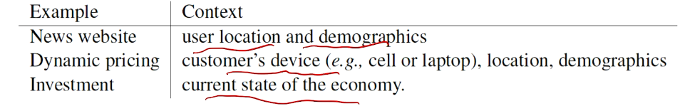
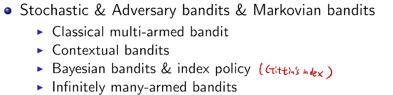
types of context
example
先验or后验
structured
global
summary
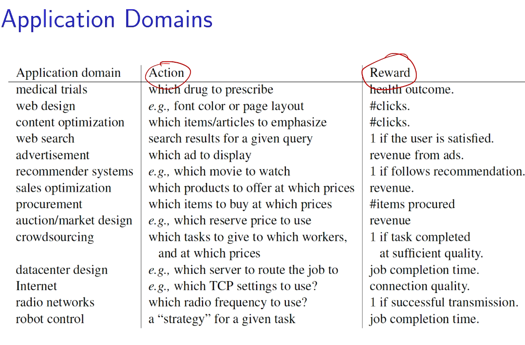
example
网飞 展示广告
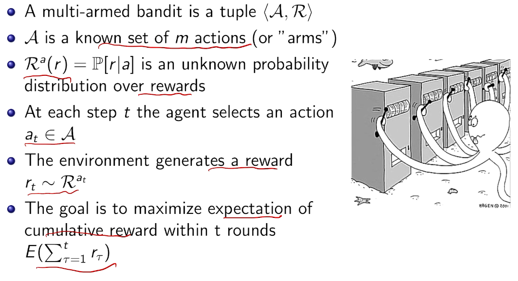
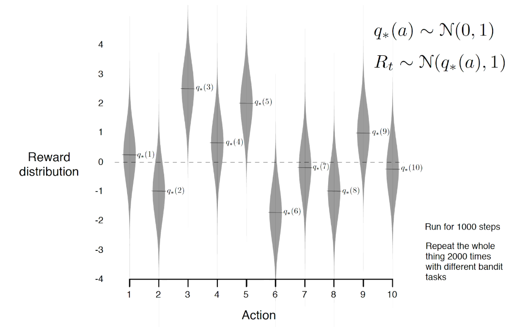
随机bandit
regret: equivalent goal
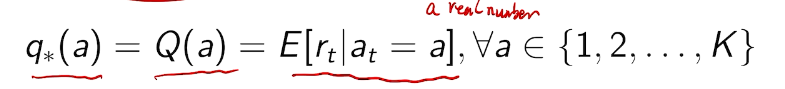
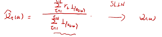
the value of an arbitrary action a is the mean reward for a (unknown):
the optimal value is 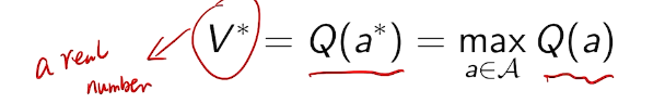
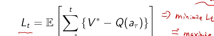
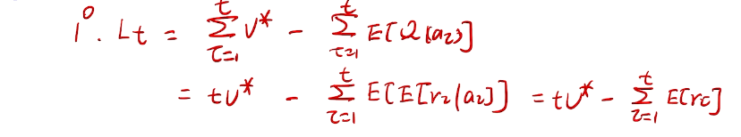
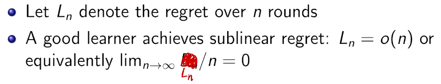
we care about total regret
example on a
In general, those values are unknown.
we must try actions to learn the action-values(explore), and prefer those that appear best(exploit).
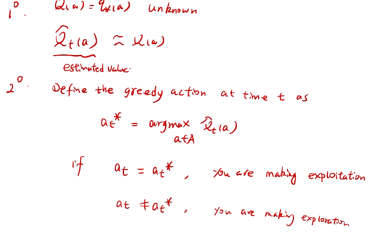
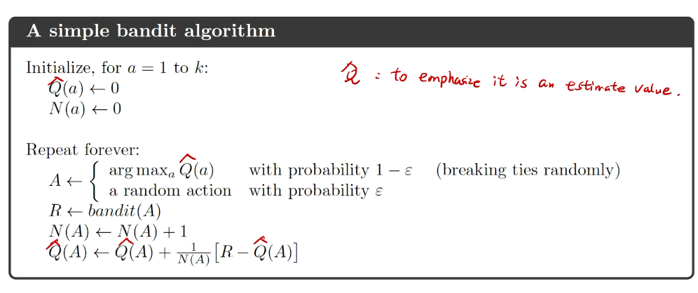
action-value methods
methods that learn action-value estimates and nothing else
根据强大数定理。收敛于真实期望值。
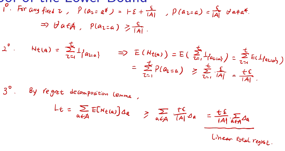
counting regret
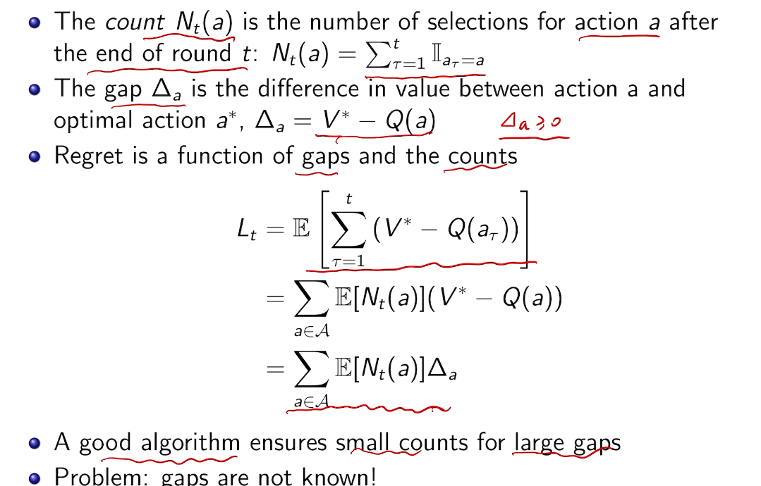
桥梁:计算total regret。 变量为指示变量
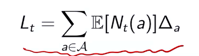
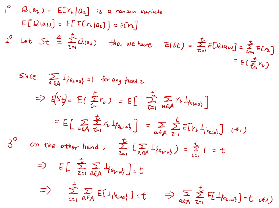

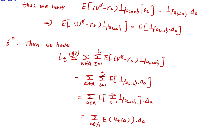
亚当定理:得到lemma的结果
how to define a good learner.
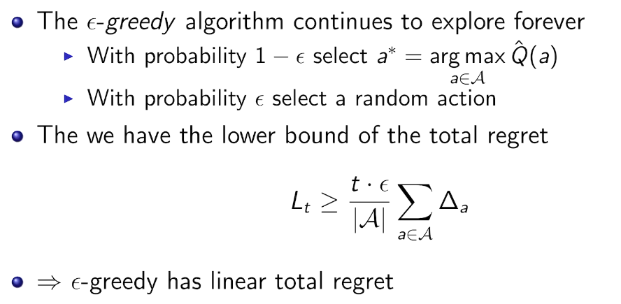
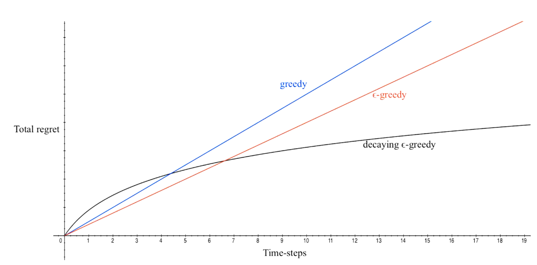
linear!! 有两种情况
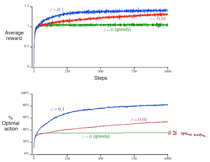
Greedy algorithm
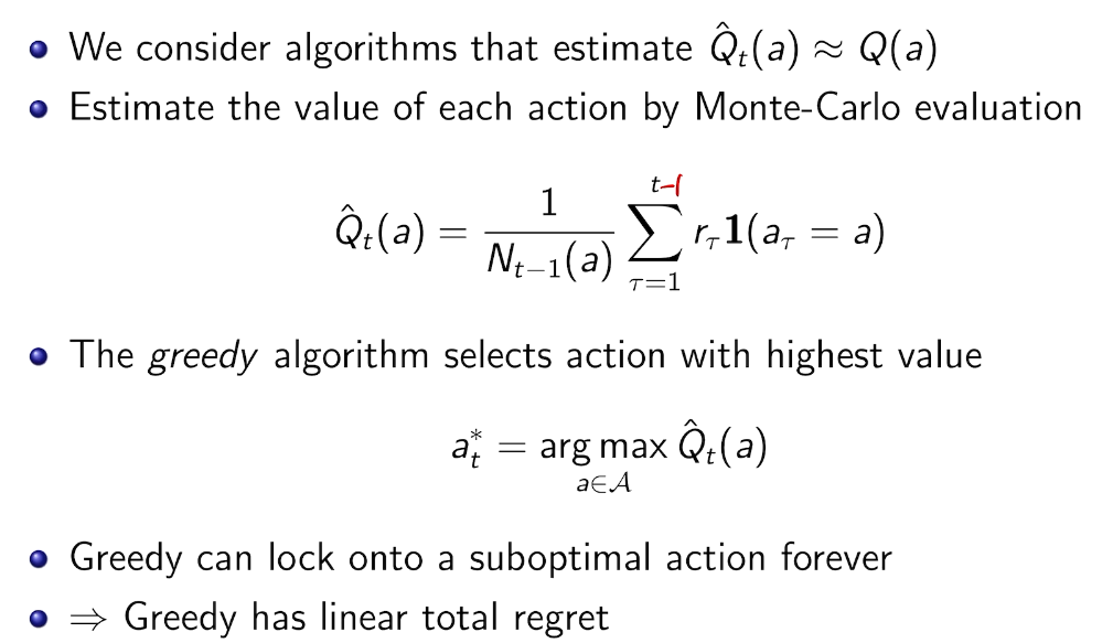
每次取最高的期望
\(\epsilon - greedy\)
防止出现局部最优
proof of lower bound
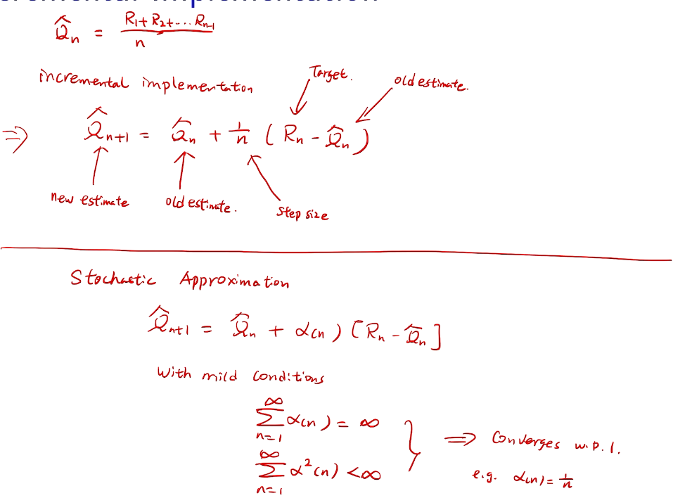
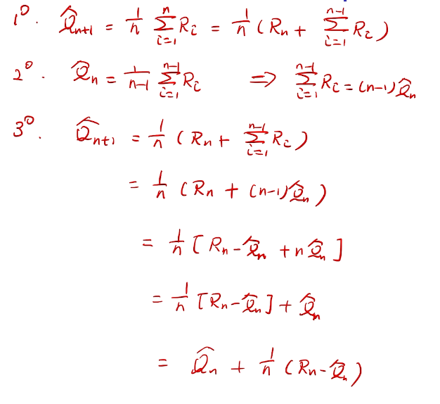
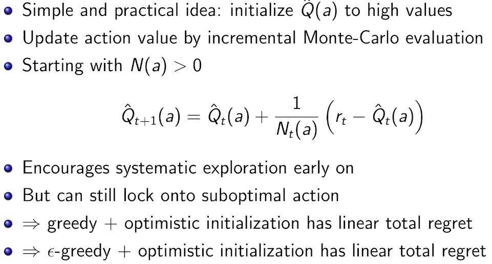
incremental implementation
性能考量、实现在线学习
proof
bandit notation
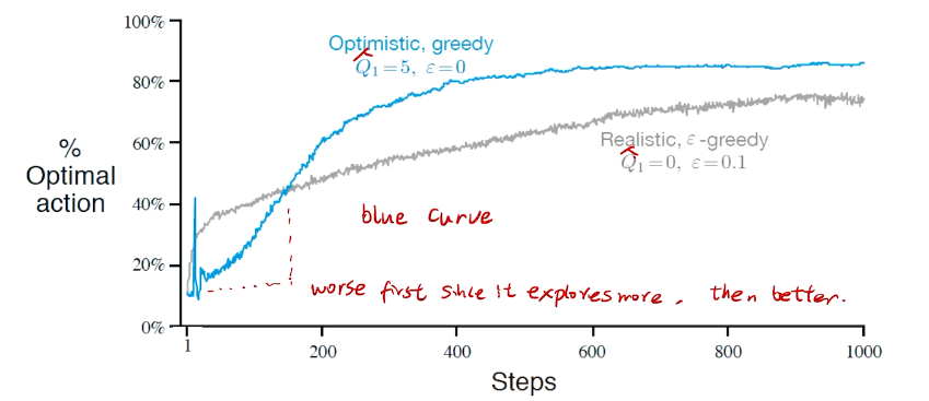
进一步提高性能 Optimistic Initial values
All methods s ofar depends on  which is 0 in this case. but we can do 5.
Initally bad case for more 尝试。
algorithm
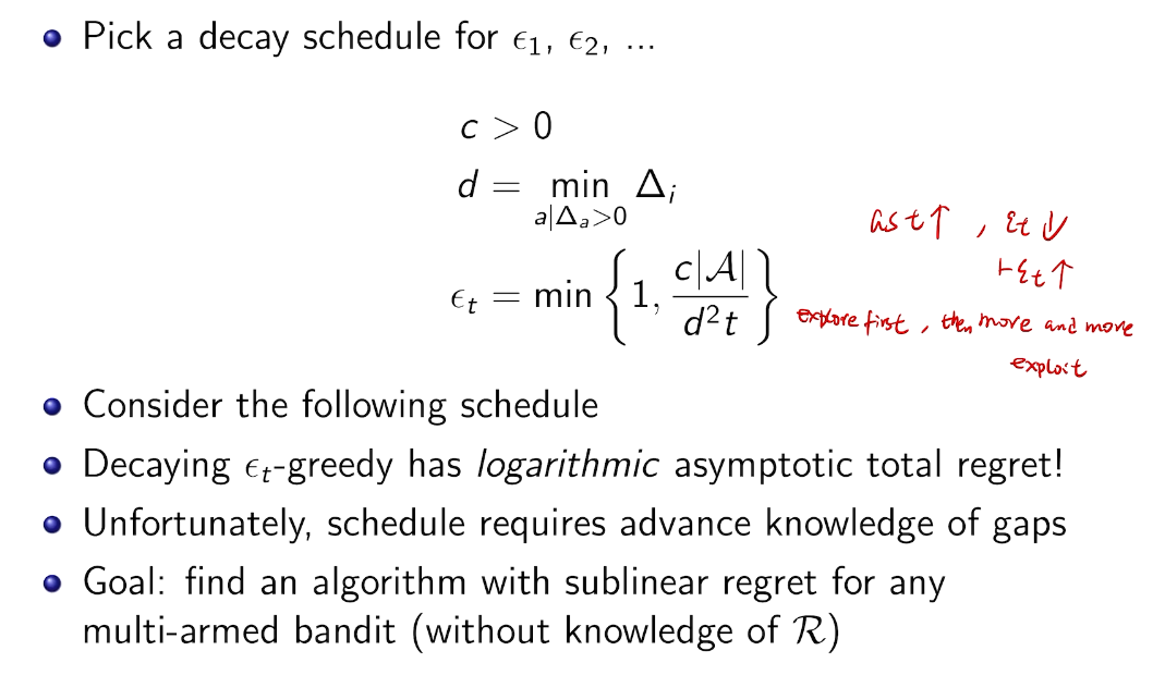
DecayIng \(\epsilon _{t} -Greedy\)
insight:先降后升
 ## bandit algorithm lower bounds(depends on gaps)
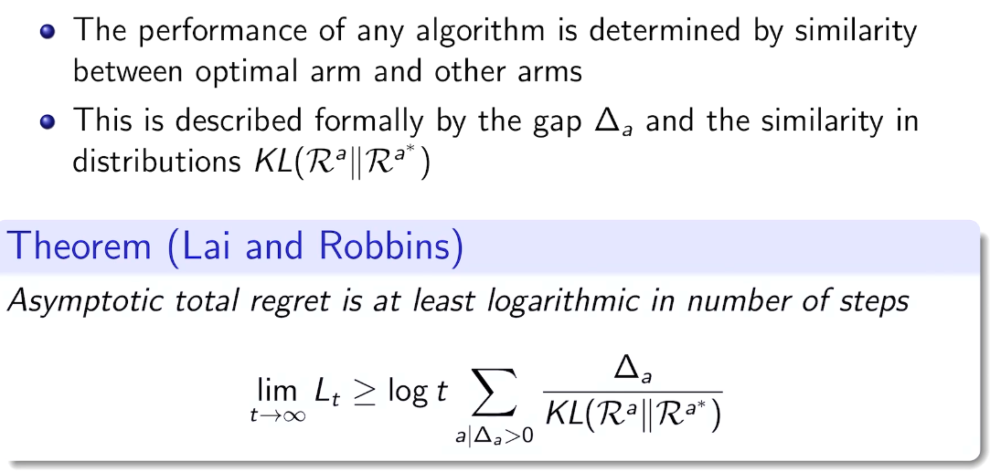
Optimism in the face of uncertainty
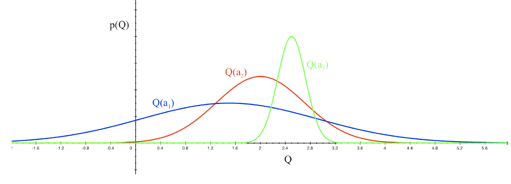
which action to pick?
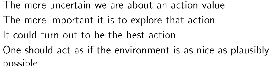
越未知需要探索
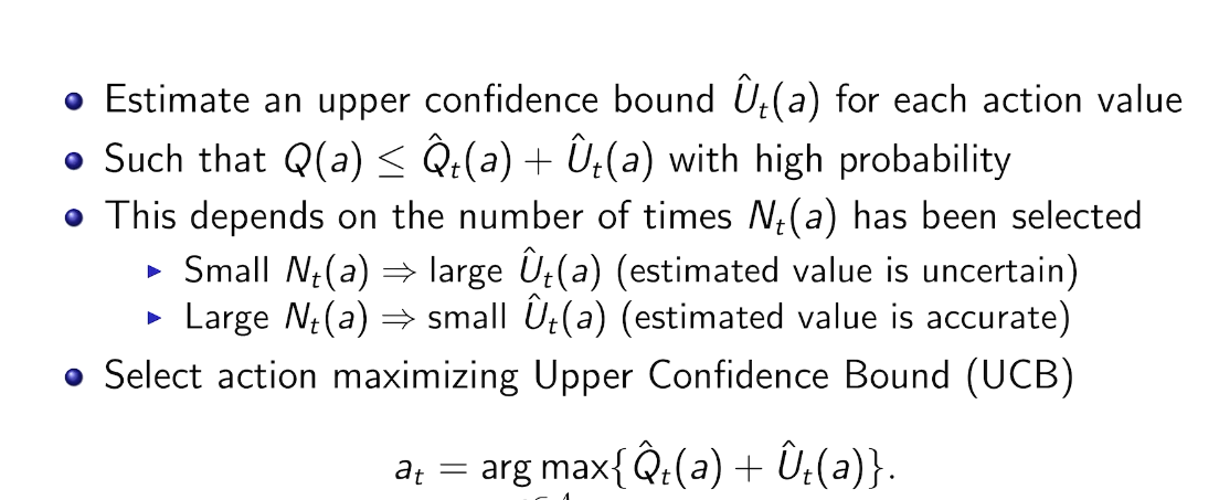
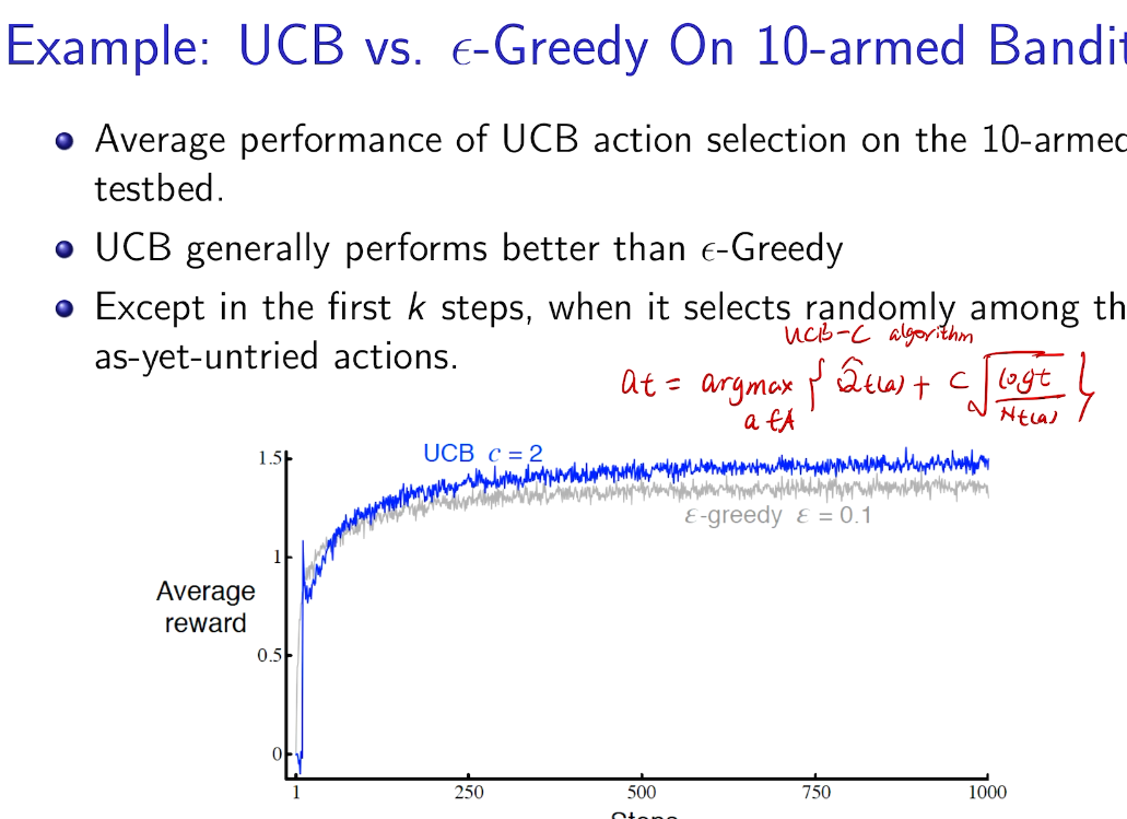
Upper Confidence Bound
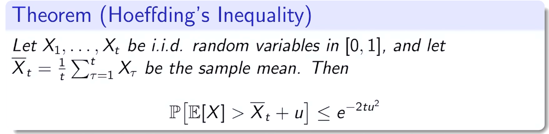
hoeffding's inequality
general case
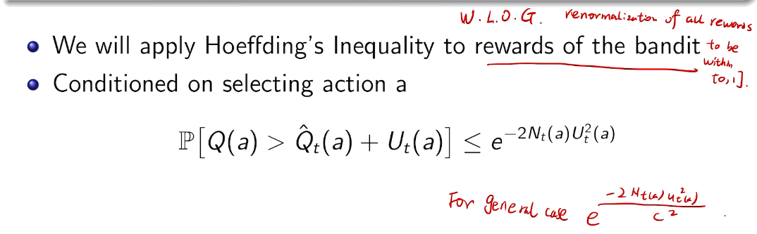
calculation
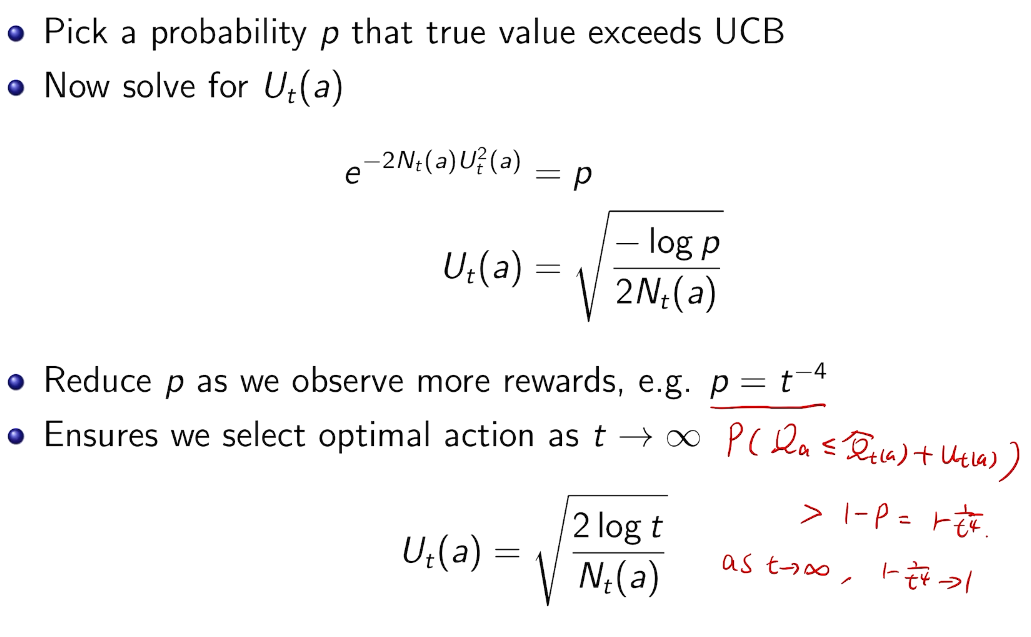
取bound得到置信区间的位置
UCB1
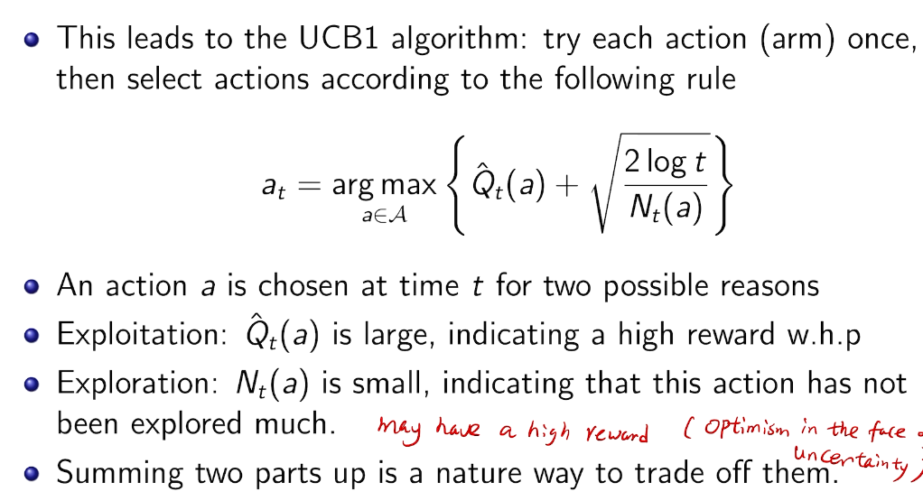
action 没有被充分的探索过,所以需要探索
上界探索
credit:https://jeremykun.com/2013/10/28/optimism-in-the-face-of-uncertainty-the-ucb1-algorithm/
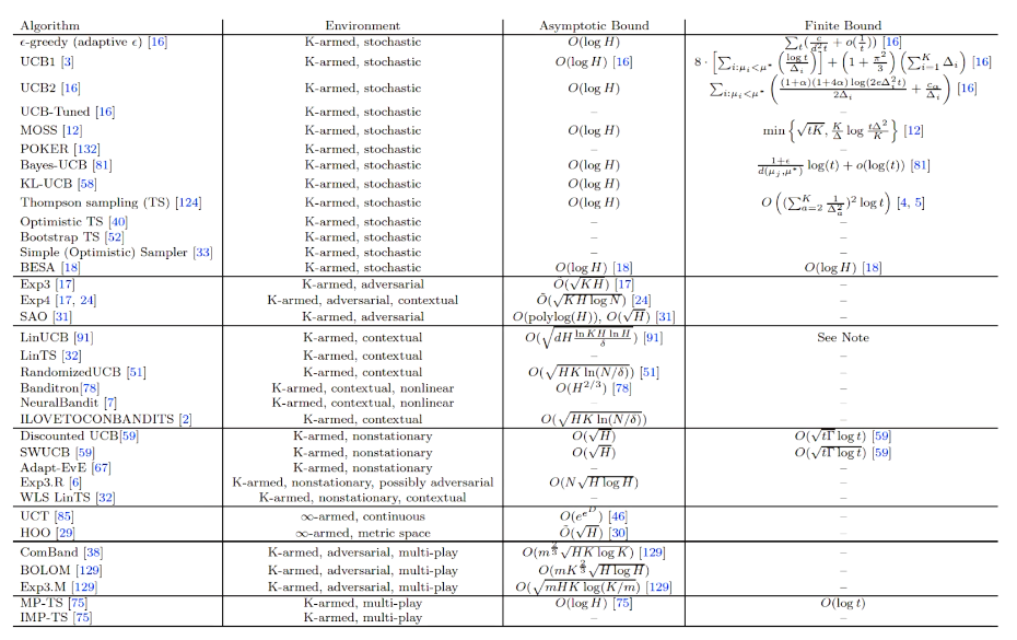
Theorem: Suppose UCB1 is run as above. Then its expected cumulative regret  is at most$\displaystyle 8 \sum_{i : \mu_i < \mu^*} \frac{\log T}{\Delta_i} + \left ( 1 + \frac{\pi^2}{3} \right ) \left ( \sum_{j=1}^K \Delta_j \right )$
Okay, this looks like one nasty puppy, but it’s actually not that bad. The first term of the sum signifies that we expect to play any suboptimal machine about a logarithmic number of times, roughly scaled by how hard it is to distinguish from the optimal machine. That is, if  is small we will require more tries to know that action
  is suboptimal, and hence we will incur more regret. The second term represents a small constant number (the $1 + \pi^2 / 3$ part) that caps the number of times we’ll play suboptimal machines in excess of the first term due to unlikely events occurring. So the first term is like our expected losses, and the second is our risk.
But note that this is a worst-case bound on the regret. We’re not saying we will achieve this much regret, or anywhere near it, but that UCB1 simply cannot do worse than this. Our hope is that in practice UCB1 performs much better.
Before we prove the theorem, let’s see how derive the 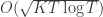 bound mentioned above. This will require familiarity with multivariable calculus, but such things must be endured like ripping off a band-aid. First consider the regret as a function
  (excluding of course
  ), and let’s look at the worst case bound by maximizing it. In particular, we’re just finding the problem with the parameters which screw our bound as badly as possible, The gradient of the regret function is given by

and it’s zero if and only if for each  ,
,  . However this is a minimum of the regret bound (the Hessian is diagonal and all its eigenvalues are positive). Plugging in the
 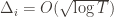 (which are all the same) gives a total bound of
  . If we look at the only possible endpoint (the
  ), then we get a local maximum of . But this isn’t the we promised, what gives? Well, this upper bound grows arbitrarily large as the
  go to zero. But at the same time, if all the
  are small, then we shouldn’t be incurring much regret because we’ll be picking actions that are close to optimal!
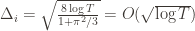
Indeed, if we assume for simplicity that all the  are the same, then another trivial regret bound is
  (why?). The true regret is hence the minimum of this regret bound and the UCB1 regret bound: as the UCB1 bound degrades we will eventually switch to the simpler bound. That will be a non-differentiable switch (and hence a critical point) and it occurs at
 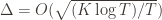 . Hence the regret bound at the switch is
 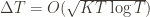 , as desired.
Proving the Worst-Case Regret Bound
Proof. The proof works by finding a bound on  , the expected number of times UCB chooses an action up to round
  . Using the
  notation, the regret is then just
  , and bounding the
  ‘s will bound the regret.
Recall the notation for our upper bound  and let’s loosen it a bit to
 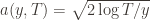 so that we’re allowed to “pretend” a action has been played
  times. Recall further that the random variable
  has as its value the index of the machine chosen. We denote by
  the indicator random variable for the event
  . And remember that we use an asterisk to denote a quantity associated with the optimal action (e.g.,
  is the empirical mean of the optimal action).
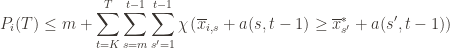
Indeed for any action  , the only way we know how to write down is as

The 1 is from the initialization where we play each action once, and the sum is the trivial thing where just count the number of rounds in which we pick action  . Now we’re just going to pull some number
  of plays out of that summation, keep it variable, and try to optimize over it. Since we might play the action fewer than
  times overall, this requires an inequality.

These indicator functions should be read as sentences: we’re just saying that we’re picking action  in round
  and we’ve already played
  at least
  times. Now we’re going to focus on the inside of the summation, and come up with an event that happens at least as frequently as this one to get an upper bound. Specifically, saying that we’ve picked action
  in round
  means that the upper bound for action
  exceeds the upper bound for every other action. In particular, this means its upper bound exceeds the upper bound of the best action (and
  might coincide with the best action, but that’s fine). In notation this event is

Denote the upper bound  for action
  in round
  by
by  . Since this event must occur every time we pick action
  (though not necessarily vice versa), we have

We’ll do this process again but with a slightly more complicated event. If the upper bound of action  exceeds that of the optimal machine, it is also the case that the maximum upper bound for action
  we’ve seen after the first
  trials exceeds the minimum upper bound we’ve seen on the optimal machine (ever). But on round
  we don’t know how many times we’ve played the optimal machine, nor do we even know how many times we’ve played machine
  (except that it’s more than
  ). So we try all possibilities and look at minima and maxima. This is a pretty crude approximation, but it will allow us to write things in a nicer form.
Denote by  the random variable for the empirical mean after playing action
  a total of
  times, and
  the corresponding quantity for the optimal machine. Realizing everything in notation, the above argument proves that

Indeed, at each  for which the max is greater than the min, there will be at least one pair
  for which the values of the quantities inside the max/min will satisfy the inequality. And so, even worse, we can just count the number of pairs
  for which it happens. That is, we can expand the event above into the double sum which is at least as large:
We can make one other odd inequality by increasing the sum to go from  to
to 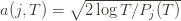 . This will become clear later, but it means we can replace
  with
with  and thus have

Now that we’ve slogged through this mess of inequalities, we can actually get to the heart of the argument. Suppose that this event actually happens, that  . Then what can we say? Well, consider the following three events:
(1) 
(2) 
(3) 
In words, (1) is the event that the empirical mean of the optimal action is less than the lower confidence bound. By our Chernoff bound argument earlier, this happens with probability  . Likewise, (2) is the event that the empirical mean payoff of action
  is larger than the upper confidence bound, which also occurs with probability
  . We will see momentarily that (3) is impossible for a well-chosen
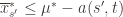
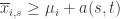
  (which is why we left it variable), but in any case the claim is that one of these three events must occur. For if they are all false, we have

and

But putting these two inequalities together gives us precisely that (3) is true:

This proves the claim.
By the union bound, the probability that at least one of these events happens is  plus whatever the probability of (3) being true is. But as we said, we’ll pick
  to make (3) always false. Indeed
  depends on which action
  is being played, and if
 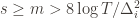 then
then  , and by the definition of
  we have
 .
.
Now we can finally piece everything together. The expected value of an event is just its probability of occurring, and so
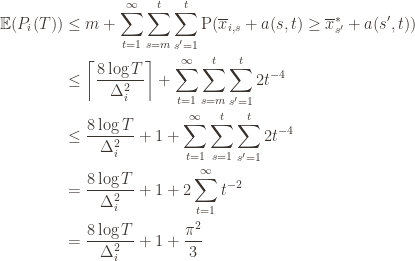
The second line is the Chernoff bound we argued above, the third and fourth lines are relatively obvious algebraic manipulations, and the last equality uses the classic solution to Basel’s problem. Plugging this upper bound in to the regret formula we gave in the first paragraph of the proof establishes the bound and proves the theorem.
result
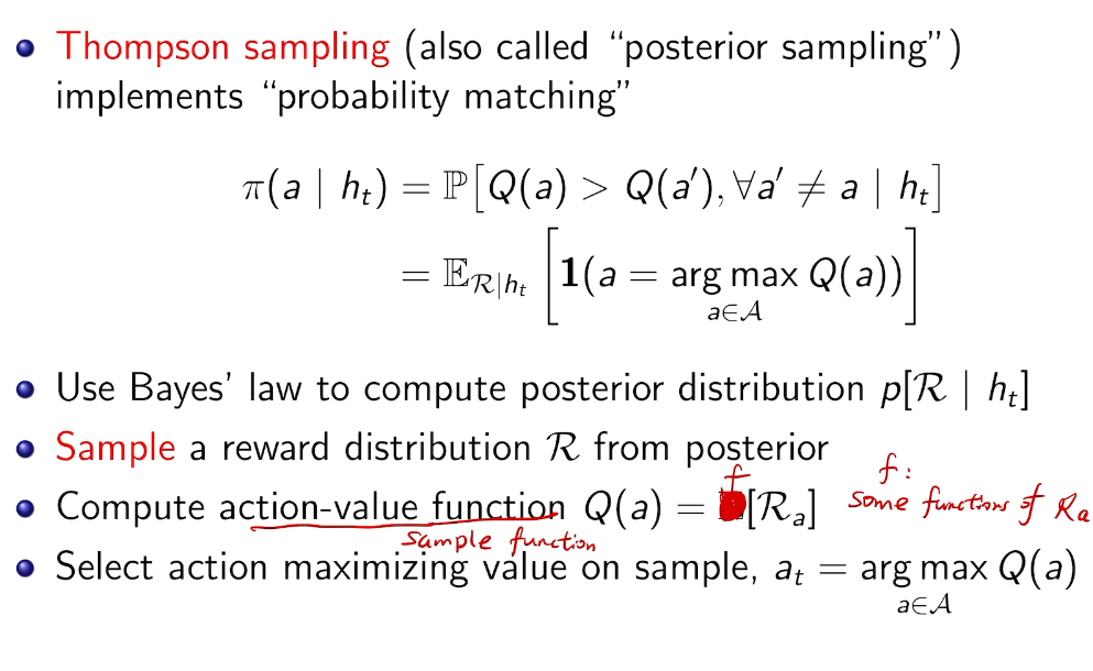
Intro for Thompson Sampling
Probability Matching
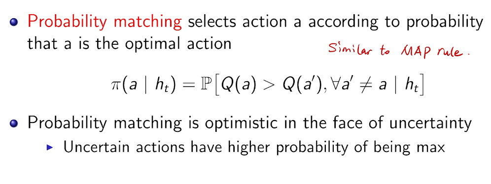
~ 最大后验概率
history
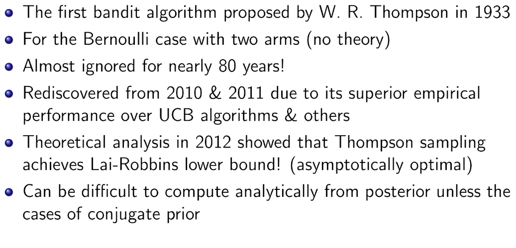
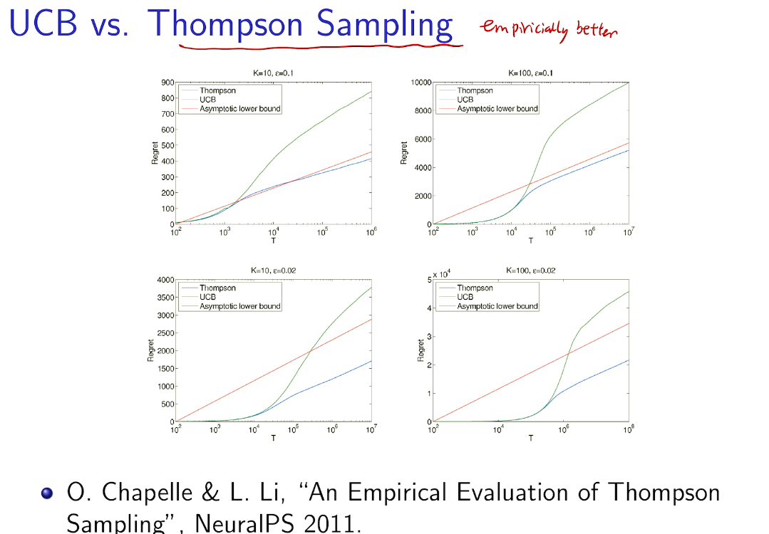
在知道后验的情况下比UCB 好
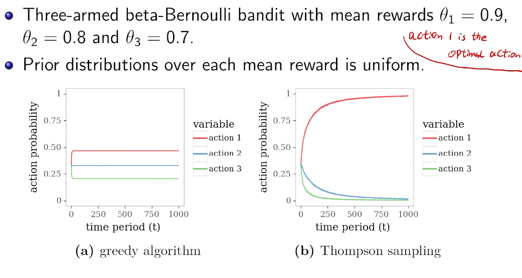
beta-bernoulli bandit
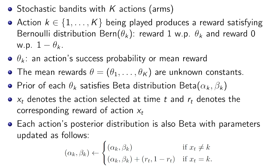
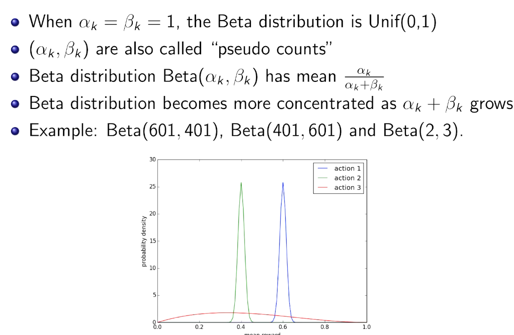
先验共轭
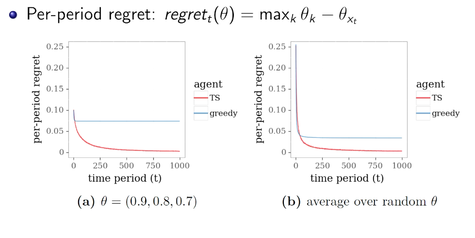
greedy vs. Thompson Sampling
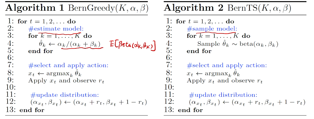
第一步不一样。 期望 vs 样本值
simulation
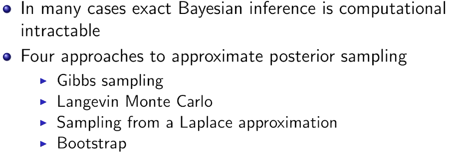
Other kind of Bayesian inference
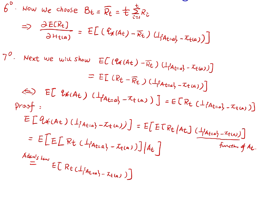
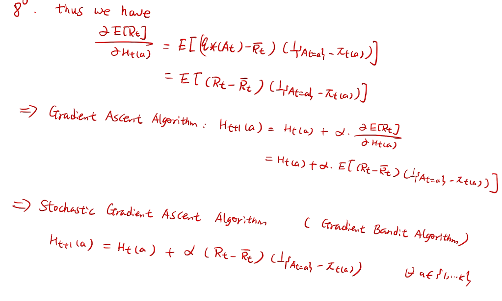
梯度bandit 算法
随机梯度上升法
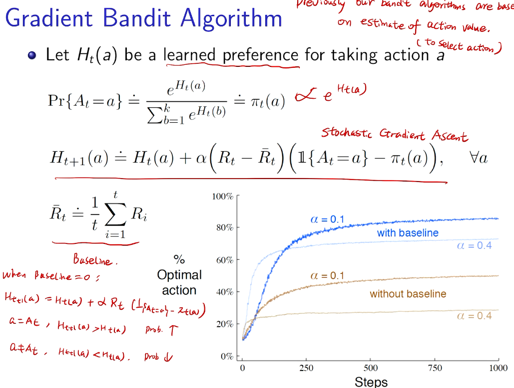
why not 梯度下降?
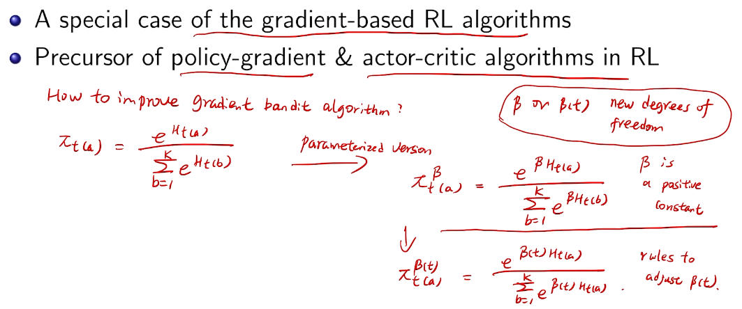
more general for RL
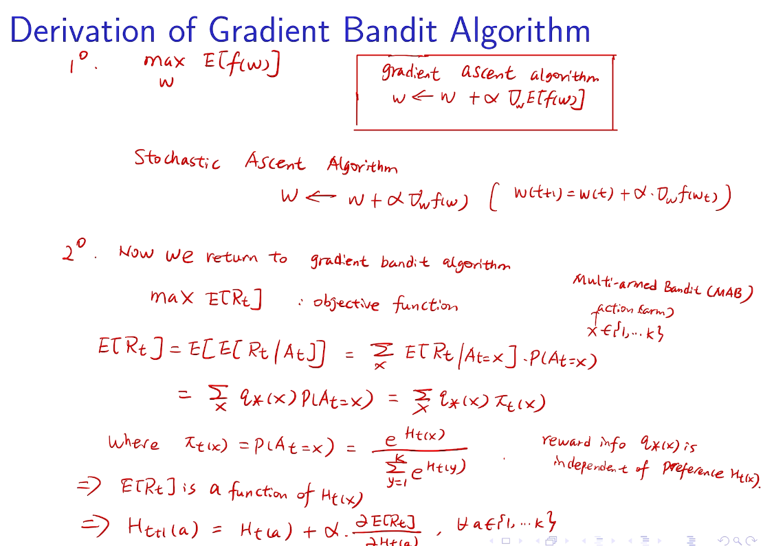
proof
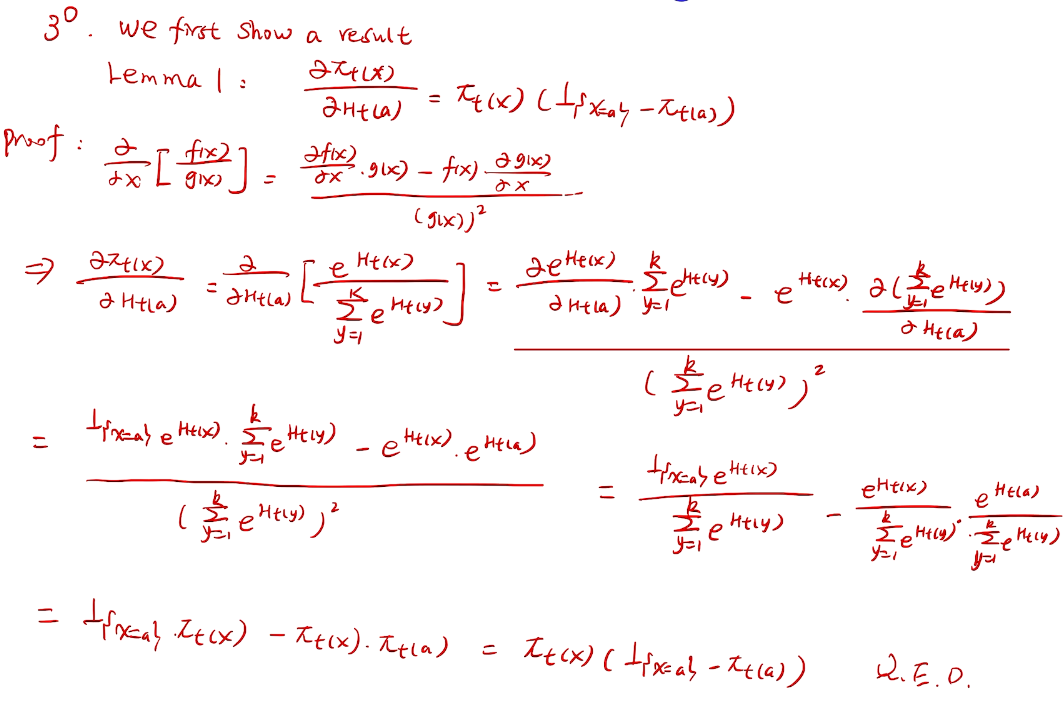
// lemma 1 for homework
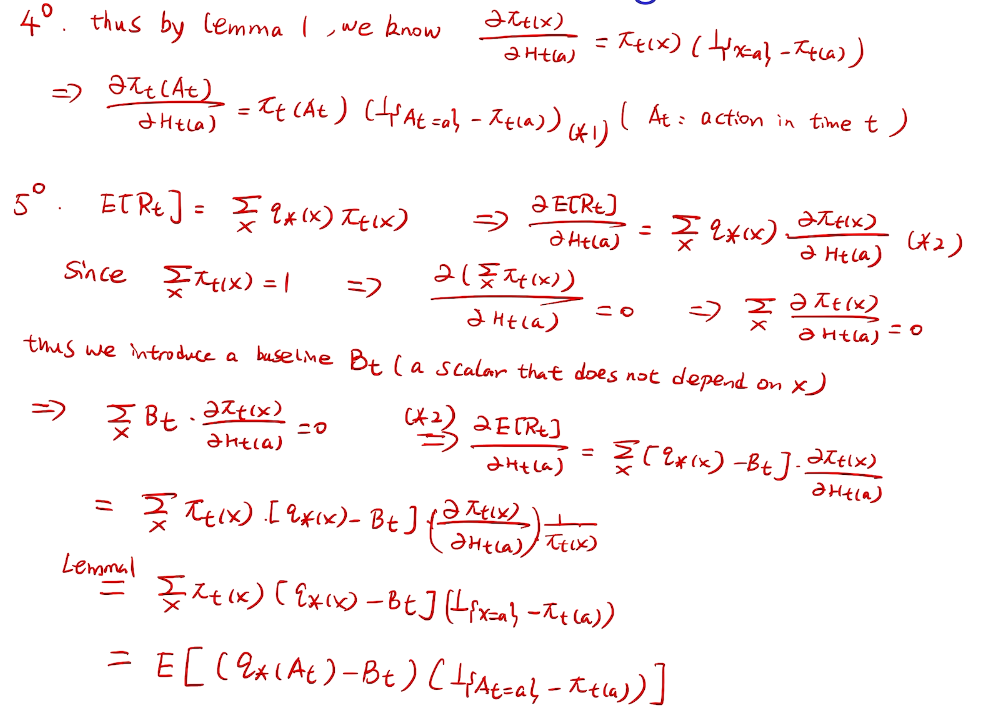
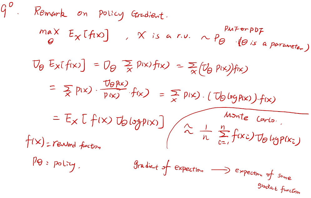
梯度的期望->期望的梯度
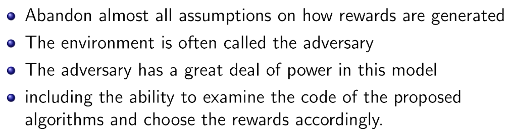
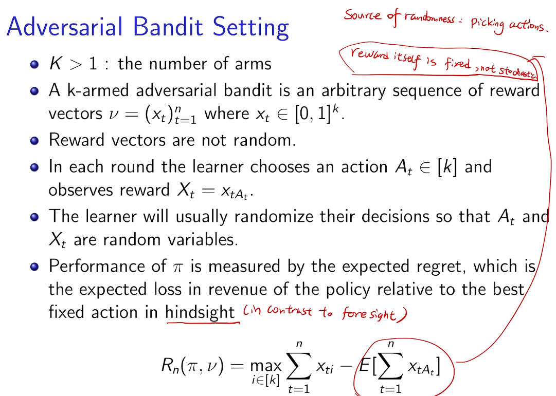
Adversarial Bandit
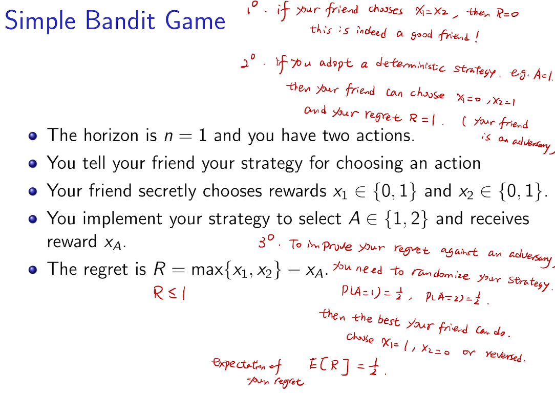
simple bandit game
importance-weighted estimators
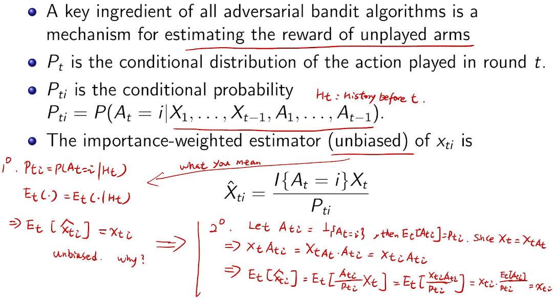
用于估计其他未被触发的arm
another good algorithm
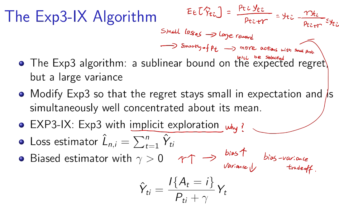
bias ~ variance tradeoff
方差太大。
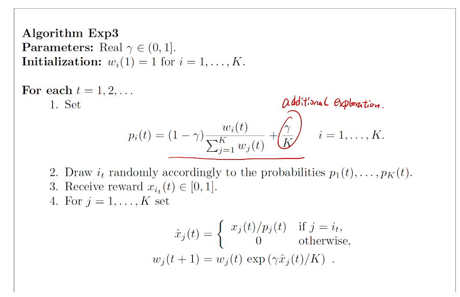
几率小的reward 现在增大了。 用隐含的增加的探索来使反差减少
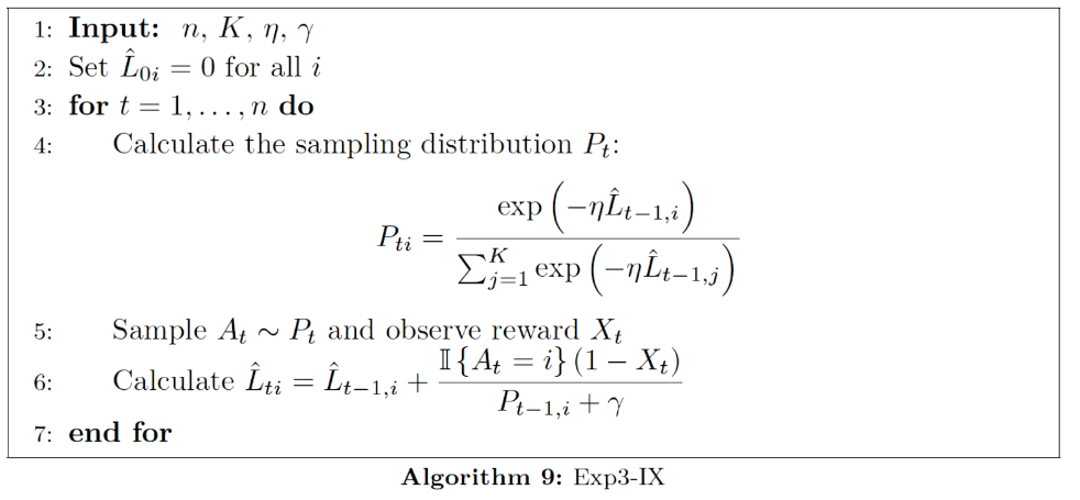
algorithm
adversary bandits with expert's advice
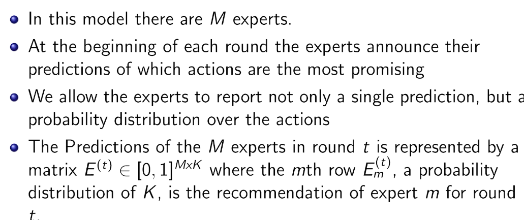
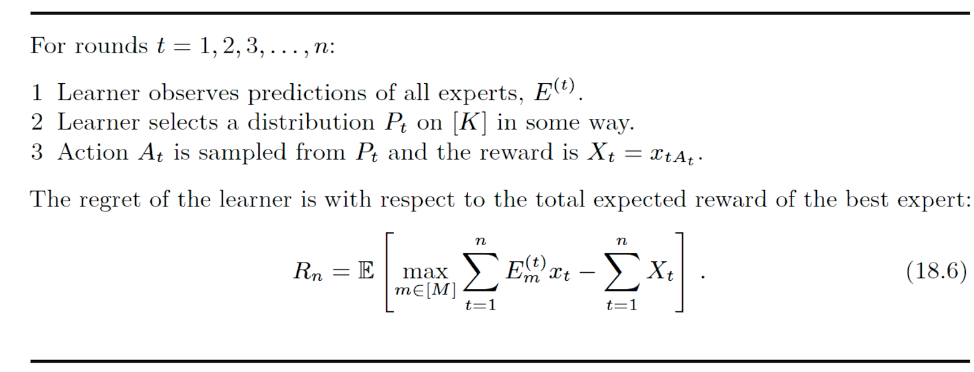
意见的权重的分布=》exp4
additional exploration
uniform exploration
proved no need
summary
bound
看作为独立为RL之外的眼界方向


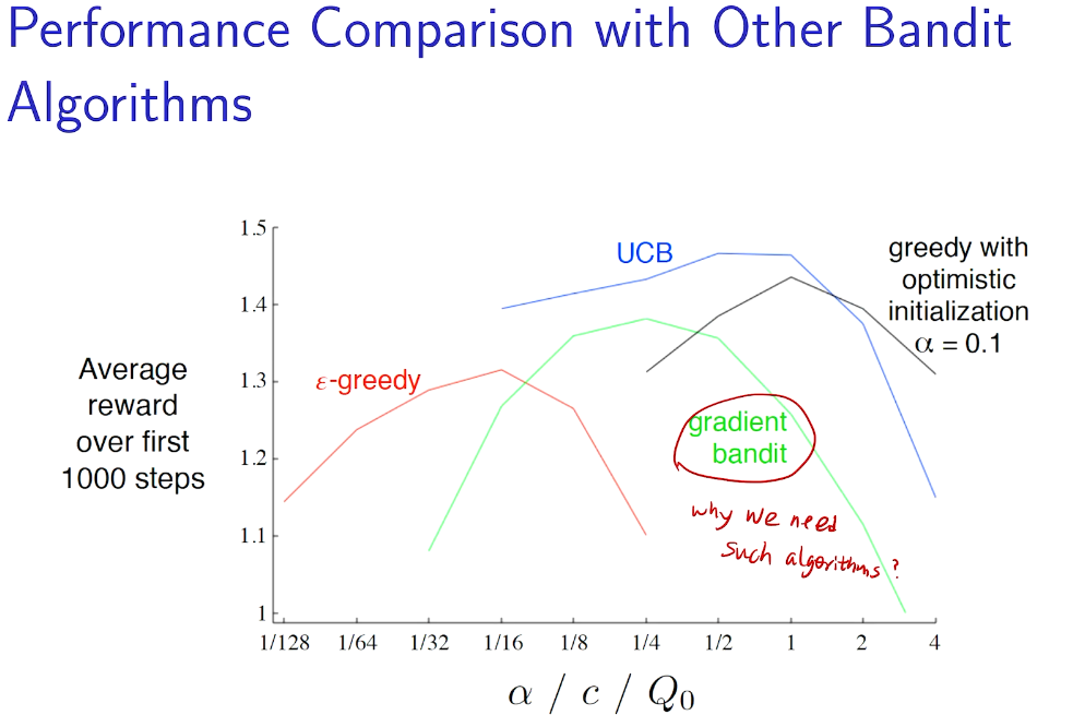
 vs
vs