One of the most import algorithm in the new century
Intro to the fft
The basic equation of the FFT
\(F(\omega)=F|f(t)|=\int ^{+\infty}_{-\infty}f(t)e^{-j\omega t}dt\)
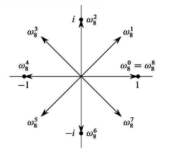
Roots of unity
\[
\begin{array}{l}\text { An n'th root of unity is an } \omega \text { s.t. } \ \omega^{n}=1 \text { . } \ \text { There are n roots n'th roots of } \ \text { unity, and they have the form } \ e^{\frac{2 \pi i k}{n}}, \text { for } 0 \leq k \leq n-1 \text { . } \ \text {Write } \omega_{n}=e^{\frac{2 \pi i}{n}} \text { , so that the n'th } \ \text { roots of unity are } \omega_{n}^{0}, \omega_{n}^{1}, \ldots, \omega_{n}^{n-1} \end{array}\]
Some problems to differ DT,DFT,FFT,IFFT
They are Fourier Transform, Discrete Fourier Transform, Fast Fourier Transform and Inverse Fourier Transform.
The transform factor:
\(\text { Fact } 1 \omega_{n}^{n}=1 \text { . } \ \text { Fact } 2 \omega_{n}^{k+\frac{n}{2}}=-\omega_{n}^{k} \ \text { Fact } 3\left(\omega_{n}^{k}\right)^{2}=\omega_{n}^{2 k}=\omega_{n / 2}^{k}\)
Why we should have the DFT.
Because in theory, all the data stored in computer is Discrete. So we have to use the equation \(X(k)=\sum^{N-1}_0x(n)W^{kn}_N(k\in \mathbb{N})\)
The Transform factor is used to prove the
1) Periodicity
\(W_{N}^{m+l N}=W_{N}^{m},\)\) where \(\(: W_{N}^{-m}=W_{N}^{N-m}\)
2) Symmetry
\(W_{N}^{m+\frac{N}{2}}=-W_{N}^{m}\)
3) Contractability
\(W_{N / m}^{k}=W_{N}^{m k}\)
4) Special rotation factors
\(W_{N}^{0}=1\)
- Why Fourier Fast Algorithm (aka FFT)?
FFT is a DFT-based algorithm designed to accelerate the computational speed of DFT.
Given a degree \(n\) -1 polynomial
\(A(x)=a_{0}+a_{1} x+a_{2} x^{2}+\dots+a_{n-1} x^{n-1}\)
DFT computes \(A\left(\omega_{n}^{0}\right), A\left(\omega_{n}^{1}\right), \ldots, A\left(\omega_{n}^{n-1}\right)\)
since \(A(x)=a_{0}+x\left(a_{1}+x\left(a_{2}+\cdots\right) \ldots\right)\)
\(A(x)\) can be evaluated in \(\mathrm{O}(\mathrm{n})\) time and
\(\mathrm{O}(1)\) memory.
- DFT can be computed trivially in \(\mathrm{O}\left(\mathrm{n}^{2}\right)\)
time.
For the DFT formula computer implementation the complexity is o(N²), while the complexity by FFT calculation is reduced to: N×log2(N)
- What is the sequence split extraction in FFT?
The sequence splitting process of FFT is the extraction process, which is divided into: extraction by time and extraction by frequency.
1) Extraction by time (also called parity extraction)
2) Frequency, which we don’t apply here.
- How does FFT reduce the amount of computation?
In simple terms, mathematicians use the above mentioned properties of the rotation factor W such as periodicity, symmetry, etc. to simplify the formula. In algorithmic programming, new points are constantly counted using points that have already been counted, i.e., old points count new points.
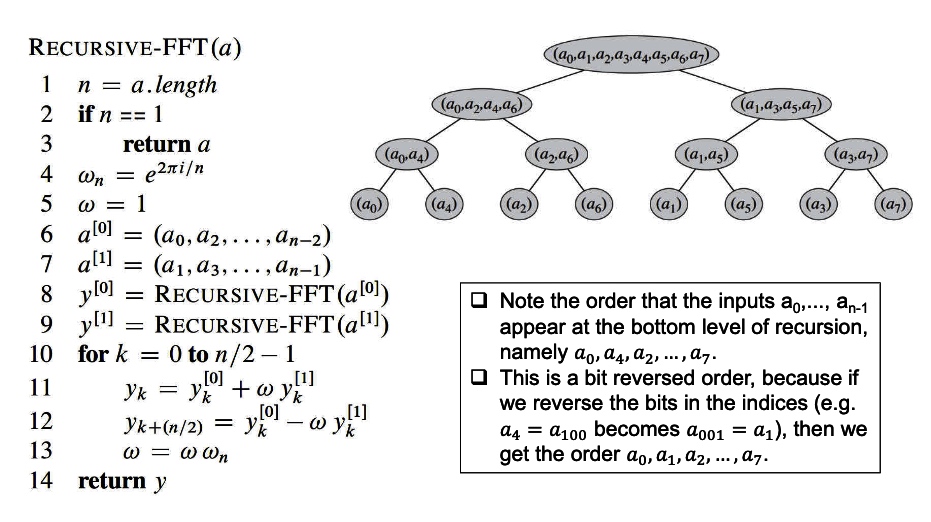
Theoretically, FFT computes the DFT in O(n log n) time using divide and conquer.
\square Suppose n is a power of 2.
Let \(A^{[0]}=a_{0}+a_{2} x^{1}+a_{4} x^{2}+\cdots+a_{n-2} x^{\frac{n}{2}-1}\)
\(A^{[1]}=a_{1}+a_{3} x^{1}+a_{5} x^{2}+\cdots+a_{n-1} x^{\frac{n}{2}-1}\)
Then \(A(x)=A^{[0]}\left(x^{2}\right)+x A^{[1]}\left(x^{2}\right)\).
So can compute \(A\left(\omega_{n}^{0}\right), A\left(\omega_{n}^{1}\right), \ldots, A\left(\omega_{n}^{n-1}\right)\) by computing \(A^{[0]}\) and \(A^{[1]}\)
at \(\left(\omega_{n}^{0}\right)^{2},\left(\omega_{n}^{1}\right)^{2}, \ldots,\left(\omega_{n}^{n-1}\right)^{2}\), and multiplying some terms by
\(\omega_{n}^{0}, \omega_{n}^{1}, \ldots, \omega_{n}^{n-1}\).
But \(\left(\omega_{n}^{k+n / 2}\right)^{2}=\omega_{n}^{2 k+n}=\omega_{n}^{2 k}=\left(\omega_{n}^{k}\right)^{2}\) by Fact 1.
A So \(\left\{\left(\omega_{n}^{0}\right)^{2},\left(\omega_{n}^{1}\right)^{2}, \ldots,\left(\omega_{n}^{n-1}\right)^{2}\right\}=\left\{\left(\omega_{n}^{0}\right)^{2},\left(\omega_{n}^{1}\right)^{2}, \ldots,\left(\omega_{n}^{n / 2-1}\right)^{2}\right\},\) i.e. only need
to evaluate \(A^{[0]}\) and \(A^{[1]}\) at n/2 points instead of n.
Also, \(\left(\omega_{n}^{k}\right)^{2}=\omega_{n}^{2 k}=\omega_{n / 2}^{k}\)
Note: Simply splitting a multipoint sequence into a less point sequence without simplification is not a reduction in arithmetic volume!!! Splitting is only in the service of simplification, using the spin factor is the key to arithmetic reduction!!!
Time Complexity:
Thus, computing \(A(x)=A^{[0]}\left(x^{2}\right)+x A^{[1]}\left(x^{2}\right)\) for
\(x \in\left\{\omega_{n}^{0}, \omega_{n}^{1}, \ldots, \omega_{n}^{n-1}\right\}\) requires
\(\square\) Computing for \(A^{[0]}(x)\) and \(A^{[1]}(x)\) for \(x \in\)
\(\left\{\omega_{n / 2}^{0}, \omega_{n / 2}^{1}, \ldots, \omega_{n / 2}^{n / 2-1}\right\}\)
-
These are also DFT’s, so can be done recursively using two
n/2-point FFT’s.
\square For \(0 \leq k \leq \frac{n}{2}-1\)
\[
\begin{array}{l}\qquad A\left(\omega_{n}^{k}\right)=A^{[0]}\left(\omega_{n / 2}^{k}\right)+\omega_{n}^{k} A^{[1]}\left(\omega_{n / 2}^{k}\right) \ \begin{array}{l}\qquad A\left(\omega_{n}^{k+n / 2}\right)=A^{[0]}\left(\omega_{n / 2}^{k+n / 2}\right)+\omega_{n}^{k+n / 2} A^{[1]}\left(\omega_{n / 2}^{k+n / 2}\right) \ =A^{[0]}\left(\omega_{n / 2}^{k}\right)-\omega_{n}^{k} A^{[1]}\left(\omega_{n / 2}^{k}\right)\end{array}\end{array}
\]
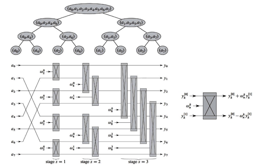
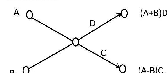
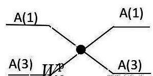
- Butterfly operation?
For a butterfly operation, you can understand it as an operation that is customizable by a graph.
The left side is the input and the right side is the output, for the letters on the horizontal line there are two cases.
1) A number on the left end line (none means C and D are 1).
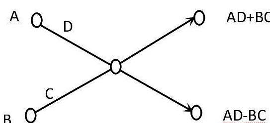
2)The right end lines have the numerical representation, but if none, C & D are 0s.
The FFT takes out odd and even in accordance to time to change the original sequence. which have to sequentialize it to make the algorithm meet the required sequence. The new sequence is the reverse binary sequence of the original ones.
For example \((a_0 a_4 a_2 a_6 a_1 a_5 a_3 a_7)\) have the binary sequence \((000,100,010,110,001,101,011,111)\).
The reverse order can be simply treated as the change of 2 near binary number, which in this case is:\((a_0 a_1 a_2 a_3 a_4 a_5 a_6 a_7)\);
Which is \((000,001,010,011,100,101,110,111)—>(000,100,010,110,001,101,011,111)\).
The code for this transformation:
for(I=0;I<N;I++) // According to law 4, you need to perform inter-code inverse order for all elements of the array
{
  /* Get the value of the inverse J of subscript I*/
  J=0;
  for(k=0;k<(M/2+0.5);k++) //k indicates operation
     {
        /* Reverse sequence operation*/
        m=1;//m is a binary number with a minimum of 1
        n=(unsigned int)pow(2,M-1);//n is a binary number with the Mth degree of 1.
        m <<= k; // for m move left k
        n>>= k; //shift k bits to the right of n
        F0=I & n;//I & n by the kth position of the first half of the extracted
        F1=I & m;//I with m-pressure bit corresponding to the lower part of the second half of the extracted F0
        if(F0) J=J | m; //J and m are in position or so that F0 corresponds to a low position of 1
        if(F1) J=J | n; //J and n are in the same position or so that F1 corresponds to a high level of 1
     }
   if(I<J)
    {
      Temp=A[I];
      A[I] =A[J];
      A[J]=Temp;
    }
}
The butter fly operation:
Now let’s imagine that if we want to program the FFT algorithm, the most basic implementation of the FFT algorithm is the butterfly operation, for any butterfly such as.
When N=8.
As can be seen from the above figure, to perform the butterfly operation, we have to solve the following problems.
\(\left\{\begin{array}{l}T_{R}=X_{R}(\mathrm{j}+B) \cos \frac{2 \pi}{N} p+X_{I}(j+B) \sin \frac{2 \pi}{N} p \cdots(1) \ T_{\mathrm{I}}=X_{I}(j+B) \cos \frac{2 \pi}{N} p-X_{R}(j+B) \sin \frac{2 \pi}{N} p \cdots(2) \ \mathrm{A}_{\mathrm{R}}(\mathrm{j})=X_{R}(\mathrm{j})+T_{R} \ \mathrm{A}_{\mathrm{I}}(\mathrm{j})=X_{I}(\mathrm{j})+T_{\mathrm{I}} \ \mathrm{A}_{\mathrm{R}}(\mathrm{j}+\mathrm{B})=X_{R}(\mathrm{j})-T_{R}(5) \ \mathrm{A}_{\mathrm{I}}(\mathrm{j}+\mathrm{B})=X_{I}(\mathrm{j})-T_{\mathrm{I}}(6)\end{array}\right.\)
for(L=1; L<=M;L++) //FFT butterfly level L from 1--M
{
  /* L-level operations*/
  //First calculate the interval B = 2^(L-1);
  B = 1;
  B = (int)pow(2,L-1);
  for(j=0; j<=B-1;j++)
  {
    /* Homogeneous butterfly operation*/
    // First increment k=2^(M-L)
    k = (int)pow(2,M-L);
    // Calculate the rotation index p in increments of k, then p = j*k
    P=1;
    P=j*k;
    for(i=0; i<=k-1;i++)
    {
      /* Perform butterfly operations*/
      //Array calibrated to r
      r=1;
      r=j+2*B*i;
      Tr=dataR[r+B]*cos(2.0*PI*p/N) + dataI[r+B]*sin(2.0*PI*p/N);
      Ti=dataI[r+B]*cos(2.0*PI*p/N) - dataR[r+B]*sin(2.0*PI*p/N);
      dataR[r+B]=dataR[r]-Tr;
      dataI[r+B]=dataI[r]-Ti;
      dataR[r]=dataR[r]-Tr; dataI[r+B]=dataI[r]-Ti; dataI[r]-Ti; dataR[r]=dataR[r]+Tr;
      dataI[r]=dataI[r]]+Ti;
    }
  }
}
IFFT is the reverse of the above operation.
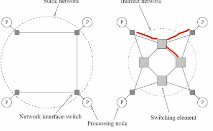
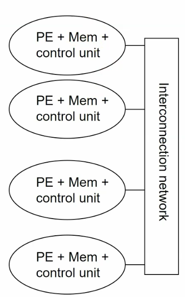
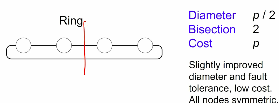
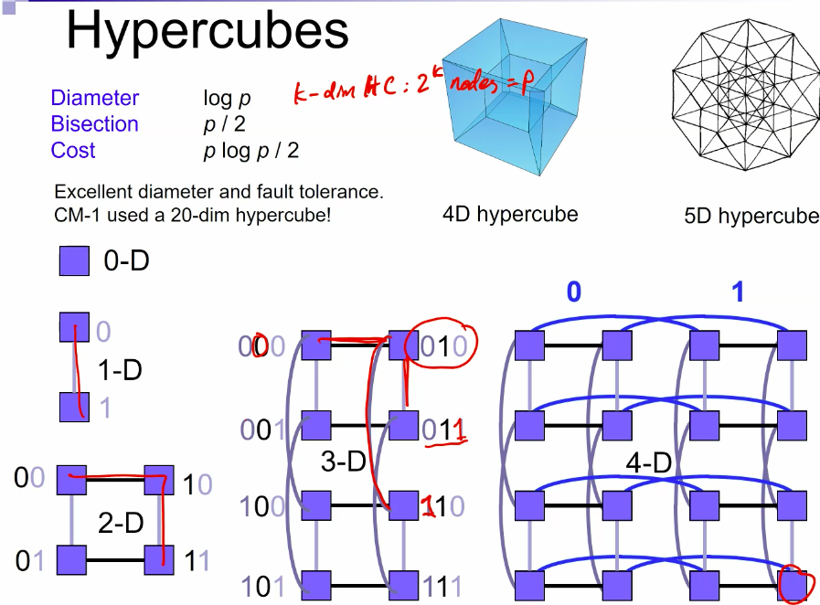
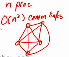
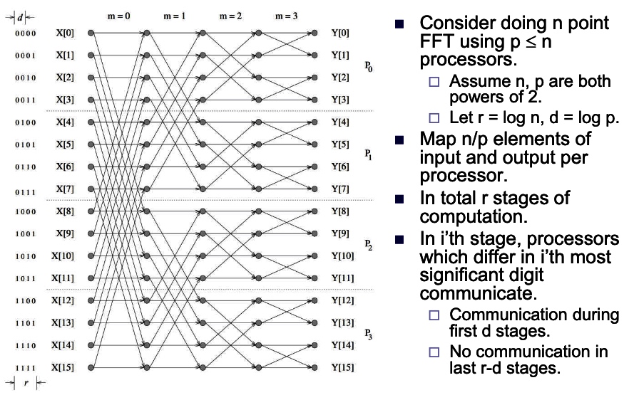
- What if we take it on the mesh or hypercube to make it scalable on gpu oprations?
Hpercube:
- Consider the binary exchange algorithm on a hypercube architecture.
- Each processor connected to d others, which differ in each digit of ID.
- Communication only with neighbors, send n/p values each time.
- since d = log p rounds of communication, communication time \(T_{c}=\) \(t_{s} \log p+t_{w} \frac{7}{p} \log p .\)
- Each stage does n/p computation.
- Total computation time \(T_{p}=\frac{t_{c} n}{p} \log n\).
- Efficiency is \(E=\frac{T_{p}}{T_{p}+T_{c}}=1 /\left(1+\frac{t_{s} p \log p}{t_{c} n \log n}+\frac{t_{w} \log p}{t_{c} \log n}\right)\)
- Define \(K\) such that \(E=1 /(1+1 / K) .\)
- For isoefficiency, want last two terms in denominator to be constant.
- \(\frac{t_{s} p \log p}{t_{c} n \log n}=\frac{1}{K}\) implies \(n \log n=W=K \frac{t_{s}}{t_{c}} p \log p .\)
- \(\frac{t_{w} \log p}{t_{c} \log n}=\frac{1}{K}\) implies \(\log n=K_{t_{c}}^{t_{w}} \log p,\) so \(n=p^{K t_{w} / t_{c}},\) so
- \(W=K \frac{t_{w}}{t_{c}} p^{K t_{w} / t_{c}} \log p\)
The efficiency for this case depends on \(t_c,t_s,t_w\), the wait time is the tradeoffs between two different lines. which is: 
From the Efficiency law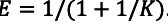
, we have once \(\frac{Kt_w}{t_c}>1\), the increasing time is polynomial with regard to the processor count.
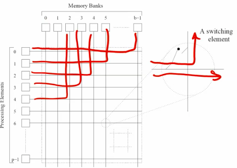
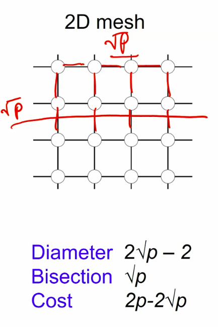
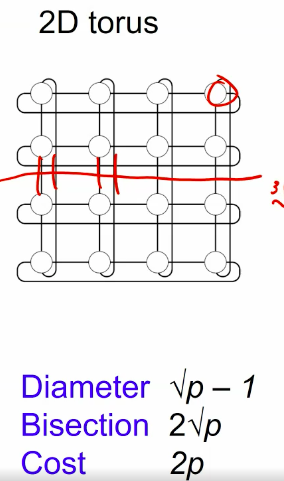
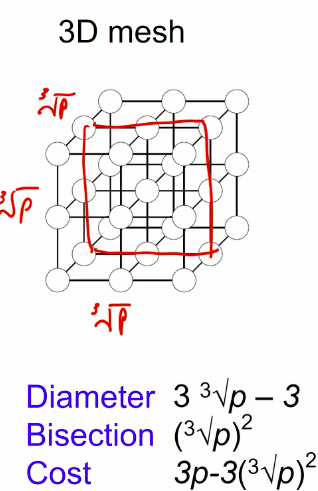
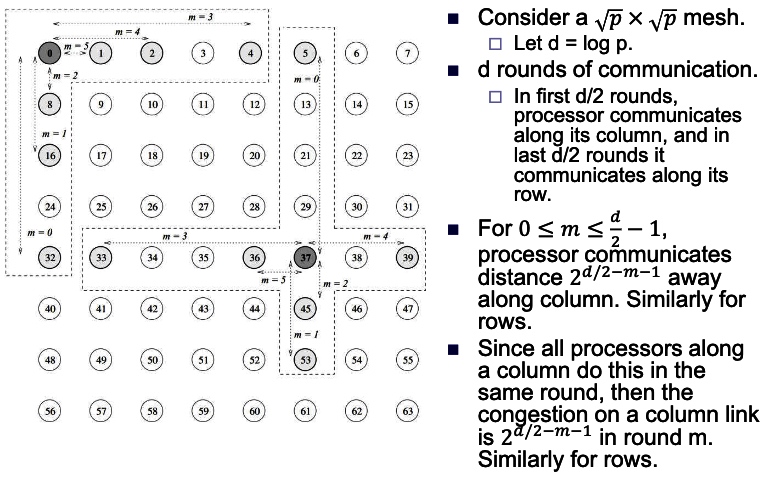
Mese:
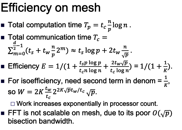
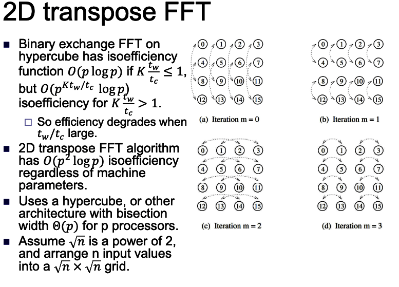
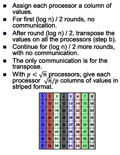
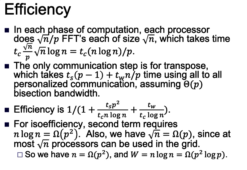
2D transpose FFT: The best:
Reference
- Prof Fan’s PPT
- Implement FFT in C by GoKing
- Implement FFT on QPU rpi3b+ by Andrew Holme